GraspForce Measurement Exercise
Load the “GraspForce” data that you acquired in Experiment 2. In this experiment, you will compute each of the short-time analysis features (as in Exercise 1) and correlate them with the force signal using linear regression. Then we will use goodness of fit measurements to show the quality of the estimate obtained through linear regression.
Implementation hints: The force signal should be normalized such that the minimum value is zero and the maximum value (corresponding to the maximum voluntary contraction or MVC) is 1. All the features should be similarly normalized.
It is important that the features are computed only in regions where there is significant force being applied. For this, you can threshold the force signal using a low value, and create a binary variable that contains a ‘1’ over the regions where there is force being applied. Use this variable to isolate regions (or segments) in both the force and EMG signal. For each segment identified, compute the mean value of each of the features, as well as the mean force value.
Normalized Force Signal as Subplots
Exercise 2.1: Using a window size of your choice:
a) Create a figure showing the EMG and normalized force signal as subplots, and indicate the regions/segments on each signal where the force is being applied and are used for your calculations.
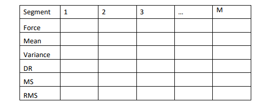
b) Create a table like the one below and populate with your results. Note this should contain the mean values for the force and each feature for every segment. (Note the number of segments for your analysis will be different).
c) Perform linear regression for each of the five metrics (dependent variable), and force (independent variable) based on the mean values found for every segment. Plot the true values vs. force, and show the trendline you found and include the equation for the line on the graph.
d) Compute and plot the residuals between true and estimate for each metric. What do these plots indicate for each feature? Be specific.
e) Compute the MSE and correlation coefficient for each feature and tabulate your results. Based on this table, which is the best estimator of force? Explain why and how you chose this. Also explain why this metric is good.
Generating A Plot of MSE vs. Correlation Coefficient
Exercise 2.2: For at least 20 different window sizes (i.e. 0.02s to 2s), repeat the above analysis and for the mean, MS, and RMS features, generate a plot of MSE vs. Correlation Coefficient for each window size. What is the best feature and window size? Explain your findings and results.
Solutions
Part (a)
Part (b)
| Segment | 1 | 2 | 3 | 4 | 5 | 6 |
| Force | 0.8113 | 0.1536 | 0.2377 | 0.4321 | 0.6008 | 0.7681 |
| Mean | 0.4743 | 0.4741 | 0.4742 | 0.4742 | 0.4739 | 0.4742 |
| Variance | 0.0167 | 6.8183e-04 | 0.0010 | 0.0039 | 0.0109 | 0.0158 |
| DR | [1 1408] | [1 1100] | [1 1344] | [1 1248] | [1 1164] | [1 1656] |
| MS | 3.3687e-04 | 4.3099e-04 | 3.5283e-04 | 3.8000e-04 | 4.0716e-04 | 2.8634e-04 |
| RMS | 0.4916 | 0.4748 | 0.4753 | 0.4784 | 0.4853 | 0.4905 |
MATLAB Code Script for Task 1
clc
clear all
close all
%%
%%%%%%%%% Data loading
data=readtable('GraspForce.csv'); %%%% reading data from excelsheet
data=data{:,2:3}; %%%% converting table into matrix form
EMG=data(50:length(data),1); %%%% Finger flexor data as EMG signal
F=data(50:length(data),2); %%%% Force data
%%%%%%%% Creating time signal
fs=1000;
T=1/fs;
t=linspace(0,T,length(F));
F_norm= (F - min(F)) / ( max(F) - min(F) ); %%%% normalized force data
EMG_norm=(EMG - min(EMG)) / ( max(EMG) - min(EMG) ); %%%% normalized EMG data
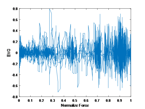
plot(F_norm,EMG)
xlabel('Normalize Force')
ylabel('EMG')
%%
%%%%%%%% Segmentation of normalozed force and normalized EMG
c=zeros(length(F_norm),1);
fori=1:length(F_norm)
ifF_norm(i,1)<= 0.1
c(i,1)=0;
else
c(i,1)=1;
end
end
y0=[];
y0=find(c(:,1)==0);
t0=[];
x=0;
fori=2:length(y0)
if y0(i,:)-y0(i-1,:)>1
x=x+1;
if x==1
t0(x,:)=i-1;
t0(x+1,:)=y0(i,:);
x=2;
elseif x>2
t0(x,:)=y0(i,:);
end
end
end
y1=[];
y1=find(c(:,1)==1);
t1=[];
z=0;
fori=2:length(y1)
if y1(i,:)-y1(i-1,:)>1
z=z+1;
t1(z,:)=y1(i,:);
end
end
%%%% Segmented normalized force
F_norm_seg1=F_norm(t0(1)+1:t0(2)-1,1);
F_norm_seg2=F_norm(t1(1):t0(3)-1,1);
F_norm_seg3=F_norm(t1(2):t0(4)-1,1);
F_norm_seg4=F_norm(t1(3):t0(5)-1,1);
F_norm_seg5=F_norm(t1(4):t0(6)-1,1);
F_norm_seg6=F_norm(t1(5):t0(7)-1,1);
%%%% Segmented normalized EMG
EMG_norm_seg1=EMG_norm(t0(1)+1:t0(2)-1,1);
EMG_norm_seg2=EMG_norm(t1(1):t0(3)-1,1);
EMG_norm_seg3=EMG_norm(t1(2):t0(4)-1,1);
EMG_norm_seg4=EMG_norm(t1(3):t0(5)-1,1);
EMG_norm_seg5=EMG_norm(t1(4):t0(6)-1,1);
EMG_norm_seg6=EMG_norm(t1(5):t0(7)-1,1);
%%
%%%%%%%%%%%%% Calculation of features
%%%% Segment 1
Force1=mean(F_norm_seg1);
Mean1=mean(EMG_norm_seg1);
Variance1=var(EMG_norm_seg1);
DR1=[1,length(EMG_norm_seg1)];
MS1=Mean1./length(EMG_norm_seg1);
RMS1=rms(EMG_norm_seg1);
seg1_metric=[Force1,Mean1,Variance1,DR1(2),MS1,RMS1];
%%%% Segment 2
Force2=mean(F_norm_seg2)
Mean2=mean(EMG_norm_seg2)
Variance2=var(EMG_norm_seg2)
DR2=[1,length(EMG_norm_seg2)]
MS2=Mean2./length(EMG_norm_seg2)
RMS2=rms(EMG_norm_seg2)
seg2_metric=[Force2, Mean2,Variance2,DR2(2),MS2,RMS2];
%%%% Segment 3
Force3=mean(F_norm_seg3)
Mean3=mean(EMG_norm_seg3)
Variance3=var(EMG_norm_seg3)
DR3=[1,length(EMG_norm_seg3)]
MS3=Mean3./length(EMG_norm_seg3)
RMS3=rms(EMG_norm_seg3)
seg3_metric=[Force3, Mean3,Variance3,DR3(2),MS3,RMS3];
%%%% Segment 4
Force4=mean(F_norm_seg4)
Mean4=mean(EMG_norm_seg4)
Variance4=var(EMG_norm_seg4)
DR4=[1,length(EMG_norm_seg4)]
MS4=Mean4./length(EMG_norm_seg4)
RMS4=rms(EMG_norm_seg4)
seg4_metric=[Force4, Mean4,Variance4,DR4(2),MS4,RMS4];
%%%% Segment 5
Force5=mean(F_norm_seg5)
Mean5=mean(EMG_norm_seg5)
Variance5=var(EMG_norm_seg5)
DR5=[1,length(EMG_norm_seg5)]
MS5=Mean5./length(EMG_norm_seg5)
RMS5=rms(EMG_norm_seg5)
seg5_metric=[Force5, Mean5,Variance5,DR1(2),MS5,RMS5];
%%%% Segment 6
Force6=mean(F_norm_seg6)
Mean6=mean(EMG_norm_seg6)
Variance6=var(EMG_norm_seg6)
DR6=[1,length(EMG_norm_seg6)]
MS6=Mean6./length(EMG_norm_seg6)
RMS6=rms(EMG_norm_seg6)
seg6_metric=[Force6, Mean6,Variance6,DR6(2),MS6,RMS6];
total_metirc=[seg1_metric;seg2_metric;seg3_metric;seg4_metric;seg5_metric;seg6_metric];
%%
%%%%%%%%%% Finding Goodness for fit measures for Segment 1
fori=2:6
b1(1,i-1)= polyfit(Force1,seg1_metric(1,i),0);
y_est1(1,i-1)=polyval(b1(1,i-1),seg1_metric(1,i));
res1(1,i-1)=seg1_metric(1,i)-y_est1(1,i-1);
mse1(1,i-1)=mean(res1(1,i-1).^2);
R1(1,i-1)=corrcoef(seg1_metric(1,i),y_est1(1,i-1));
end
%%%%%%%%%% Finding Goodness for fit measures for Segment 2
fori=2:6
b2(1,i-1)= polyfit(Force2,seg2_metric(1,i),0);
y_est2(1,i-1)=polyval(b2(1,i-1),seg2_metric(1,i));
res2(1,i-1)=seg2_metric(1,i)-y_est2(1,i-1);
mse2(1,i-1)=mean(res2(1,i-1).^2);
R2(1,i-1)=corrcoef(seg2_metric(1,i),y_est2(1,i-1));
end
%%%%%%%%%% Finding Goodness for fit measures for Segment 3
fori=2:6
b3(1,i-1)= polyfit(Force3,seg3_metric(1,i),0);
y_est3(1,i-1)=polyval(b3(1,i-1),seg3_metric(1,i));
res3(1,i-1)=seg3_metric(1,i)-y_est3(1,i-1);
mse3(1,i-1)=mean(res3(1,i-1).^2);
R3(1,i-1)=corrcoef(seg3_metric(1,i),y_est3(1,i-1));
end
%%%%%%%%%% Finding Goodness for fit measures for Segment 4
fori=2:6
b4(1,i-1)= polyfit(Force4,seg4_metric(1,i),0);
y_est4(1,i-1)=polyval(b4(1,i-1),seg4_metric(1,i));
res4(1,i-1)=seg4_metric(1,i)-y_est4(1,i-1);
mse4(1,i-1)=mean(res4(1,i-1).^2);
R4(1,i-1)=corrcoef(seg4_metric(1,i),y_est4(1,i-1));
end
%%%%%%%%%% Finding Goodness for fit measures for Segment 5
fori=2:6
b5(1,i-1)= polyfit(Force5,seg5_metric(1,i),0);
y_est5(1,i-1)=polyval(b5(1,i-1),seg5_metric(1,i));
res5(1,i-1)=seg5_metric(1,i)-y_est5(1,i-1);
mse5(1,i-1)=mean(res5(1,i-1).^2);
R5(1,i-1)=corrcoef(seg5_metric(1,i),y_est5(1,i-1));
end
%%%%%%%%%% Finding Goodness for Fit Measures for Segment 6
fori=2:6
b6(1,i-1)= polyfit(Force6,seg6_metric(1,i),0);
y_est6(1,i-1)=polyval(b6(1,i-1),seg6_metric(1,i));
res6(1,i-1)=seg6_metric(1,i)-y_est6(1,i-1);
mse6(1,i-1)=mean(res6(1,i-1).^2);
R6(1,i-1)=corrcoef(seg6_metric(1,i),y_est6(1,i-1));
end
%%%%%%%%%%%%% Table of Goodness for Fit Measures
RES=[res1;res2;res3;res4;res5;res6];
MSE=[mse1;mse2;mse3;mse4;mse5;mse6];
R=[R1;R2;R3;R4;R5;R6];
Segment_no=[1;2;3;4;5;6];
T = table(Segment_no,RES,MSE,R)