How to Solve Sparse Systems of Linear Equations Using MATLAB

Sparse systems of linear equations are widely used in engineering and scientific applications, including electrical circuit analysis, computational physics, and numerical methods for differential equations. These systems involve matrices with a large number of zero elements, which allows for efficient storage and specialized numerical algorithms. Unlike dense matrices, sparse matrices reduce computational complexity and memory usage, making them essential for solving large-scale problems. MATLAB provides powerful tools for working with sparse systems, offering both direct and iterative methods. Direct methods, such as Gaussian elimination, are effective but can become computationally expensive for large matrices. Iterative methods like the Jacobi and Gauss-Seidel methods provide an alternative approach, refining approximate solutions until convergence is achieved. These methods are particularly useful when dealing with large sparse systems where direct solvers may be impractical. This blog explores how to formulate and solve your MATLAB assignment using sparse systems, covering matrix representation, implementation of iterative methods, and convergence analysis. By comparing different approaches, students can understand the trade-offs between computational efficiency and accuracy, enabling them to choose the most suitable method for their applications. MATLAB’s built-in functions and visualization tools further enhance the ability to analyze the performance of different solvers, making it an essential tool for solving sparse systems efficiently.

Understanding Sparse Systems of Linear Equations
A system of linear equations consists of multiple linear equations that must be solved simultaneously. In mathematical form, it can be expressed as:
where A is the coefficient matrix, x is the vector of unknowns, and b is the right-hand side vector. When the coefficient matrix A has many zero elements, it is called a sparse matrix. Sparse matrices commonly arise in applications such as electrical networks, finite difference methods, finite element methods, and large-scale simulations.
Why Are Sparse Matrices Important?
The presence of numerous zero elements in a sparse matrix significantly reduces computational complexity. Instead of storing all elements, including zeros, specialized data structures in MATLAB allow storing only nonzero elements, leading to efficient memory usage. Sparse matrices also enable optimized numerical algorithms that take advantage of the sparsity pattern, improving computational efficiency compared to traditional dense matrix methods.
Formulating a Sparse System: Example of Electrical Circuits
A common real-world example of a sparse system is electrical circuit analysis, particularly in nodal voltage analysis. In this method, Kirchhoff’s Current Law (KCL) is applied to different nodes in a circuit, resulting in a system of equations where the conductance matrix is sparse.
In a typical resistor network, each node in the circuit corresponds to an unknown voltage, and the circuit connections define the coefficients of the equations. The resulting system takes the form:

where G is the conductance matrix, v is the vector of unknown voltages, and iii is the vector of independent current sources. Because each node is usually connected to only a few other nodes, the conductance matrix is sparse, making it suitable for specialized numerical techniques.
Implementing Iterative Methods in MATLAB
Solving sparse systems efficiently requires methods that do not rely on full matrix factorization. Two widely used iterative methods for solving sparse linear systems are the Jacobi and Gauss-Seidel methods. These methods provide approximate solutions by iteratively refining an initial guess until convergence is achieved.
Jacobi Method
The Jacobi method is an iterative approach that updates each unknown separately based on the previous iteration's values. The system of equations:

is rewritten such that each unknown is expressed in terms of the others:
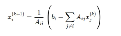
The process starts with an initial guess and iteratively updates each variable until the solution converges.
Jacobi Method Implementation in MATLAB
function x = jacobiMethod(A, b, x0, tol, maxIter)
    n = length(b);
    x = x0;
    for k = 1:maxIter
        x_new = zeros(n, 1);
        for i = 1:n
            sumVal = sum(A(i, :) * x) - A(i, i) * x(i);
            x_new(i) = (b(i) - sumVal) / A(i, i);
        end
        if norm(x_new - x, inf) < tol
            break;
        end
        x = x_new;
    end
end
This function takes the coefficient matrix A, right-hand side vector b, initial guess x0, tolerance level, and maximum number of iterations. The method stops when the difference between successive approximations is smaller than the specified tolerance.
Gauss-Seidel Method
The Gauss-Seidel method is an improvement over the Jacobi method. Instead of using only values from the previous iteration, it immediately updates and reuses newly computed values within the same iteration. The formula is:
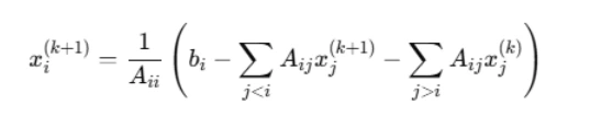
This modification usually leads to faster convergence compared to the Jacobi method.
Gauss-Seidel Method Implementation in MATLAB
function x = gaussSeidelMethod(A, b, x0, tol, maxIter)
    n = length(b);
    x = x0;
    for k = 1:maxIter
        x_old = x;
        for i = 1:n
            sum1 = sum(A(i, 1:i-1) * x(1:i-1));
            sum2 = sum(A(i, i+1:n) * x_old(i+1:n));
            x(i) = (b(i) - sum1 - sum2) / A(i, i);
        end
        if norm(x - x_old, inf) < tol
            break;
        end
    end
end
This implementation ensures that newly computed values are used immediately, improving the convergence rate.
Comparing Iterative and Direct Methods
In addition to iterative methods, sparse systems can also be solved using direct methods like Gaussian elimination. However, direct methods can be computationally expensive for large sparse matrices due to memory constraints and computational overhead.
Gaussian Elimination in MATLAB
x = A \ b;
The backslash operator in MATLAB automatically detects sparsity and applies an optimized solver. However, for very large systems, iterative methods remain preferable due to their lower memory requirements.
Convergence Analysis of Iterative Methods
To evaluate the performance of iterative methods, we compare their convergence behavior by varying the tolerance parameter. A common metric is the number of iterations required for convergence.
Performing Convergence Tests
For different tolerance levels ε=10−4,10−6,10−8,10−10, the number of iterations required to achieve convergence can be recorded. A comparison with the exact solution obtained from Gaussian elimination helps assess the accuracy.
Graphical Representation in MATLAB
eps_values = [1e-4, 1e-6, 1e-8, 1e-10];
iterations_jacobi = [];
iterations_gs = [];
error_norm_jacobi = [];
error_norm_gs = [];

for eps = eps_values
    [x_jacobi, iter_jacobi] = jacobiMethod(A, b, zeros(size(b)), eps, 1000);
    [x_gs, iter_gs] = gaussSeidelMethod(A, b, zeros(size(b)), eps, 1000);
    x_exact = A \ b;

    iterations_jacobi = [iterations_jacobi, iter_jacobi];
    iterations_gs = [iterations_gs, iter_gs];
    error_norm_jacobi = [error_norm_jacobi, norm(x_exact - x_jacobi, 2)];
    error_norm_gs = [error_norm_gs, norm(x_exact - x_gs, 2)];
end

figure;
loglog(eps_values, iterations_jacobi, '-o', eps_values, iterations_gs, '-s');
xlabel('Tolerance (\epsilon)');
ylabel('Number of Iterations');
legend('Jacobi', 'Gauss-Seidel');

figure;
loglog(eps_values, error_norm_jacobi, '-o', eps_values, error_norm_gs, '-s');
xlabel('Tolerance (\epsilon)');
ylabel('Solution Error Norm');
legend('Jacobi', 'Gauss-Seidel');
These plots illustrate how solution accuracy and computational cost depend on the tolerance parameter. Generally, Gauss-Seidel converges faster than Jacobi, but both methods require more iterations as the tolerance becomes stricter.
Conclusion
Solving sparse systems of linear equations efficiently requires both mathematical understanding and computational techniques. Sparse matrices, which contain many zero elements, appear in various scientific and engineering applications, including circuit analysis, structural mechanics, and numerical solutions to differential equations. MATLAB provides specialized tools to handle sparse matrices efficiently, allowing for reduced memory usage and faster computations compared to dense matrices.
Iterative methods such as the Jacobi and Gauss-Seidel methods are widely used for solving large sparse systems. The Jacobi method updates each unknown separately using values from the previous iteration, while the Gauss-Seidel method updates values immediately within the same iteration, leading to faster convergence. These methods offer advantages over direct methods like Gaussian elimination, which can be computationally expensive for large systems.