Effective Ways to Solve MATLAB Assignments Using Laplace Transforms, Transfer Functions, and MRI Data Processing

MATLAB assignments involving system analysis, Laplace transforms, and practical applications like MRI data processing, you may find it challenging to navigate through complex problems. However, with a clear understanding of the fundamental techniques and tools available in MATLAB, you can confidently solve your matlab assignment. This blog will guide you through a step-by-step approach that can be applied to various types of assignments. Whether you are dealing with system functions like Laplace transforms or more specialized tasks such as MRI data processing, this guide will help you solve your transfer functions assignment efficiently.
Understanding Laplace Transforms and Transfer Functions

In many engineering and control system problems, Laplace transforms play a crucial role in analyzing and modeling systems. The Laplace transform is a mathematical operation that converts a time-domain function into a frequency-domain function. This transformation makes it easier to analyze the system’s behavior, such as stability and oscillation.
When dealing with transfer functions, you are essentially defining a system’s behavior in terms of the Laplace transform. A transfer function is the ratio of the output to the input, expressed as a function of the Laplace variable s. The general form of a transfer function is given as:
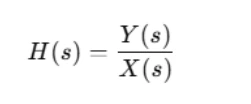
Where:
- H(s) is the transfer function,
- Y(s) is the Laplace transform of the output,
- X(s) is the Laplace transform of the input.
For example, let’s say you are given a system where the input is defined as a polynomial in s (the Laplace transform variable), and the output is also given as a polynomial in s. The first step is to write the transfer function by expressing the output and input as polynomials and taking their ratio. In MATLAB, you can define this symbolically by using the syms function to declare symbolic variables. Here's an example code:
syms s
input = 4*s^3 + 3*s^2 + 2*s + 25 + 22 + 10;  % example input
output = 4*s^4 + 5*s^3 + 95*s^2 + 50;  % example output
transfer_function = output / input;  % Transfer function
This symbolic computation allows you to define and manipulate the transfer function for further analysis. MATLAB makes it easy to visualize and analyze systems using symbolic expressions and numerical methods.
Analyzing the Transfer Function
Once you have defined the transfer function, the next step is to analyze its characteristics. The primary components of a transfer function that help in analysis are the poles, zeros, and gain. The poles are the values of s that make the denominator of the transfer function equal to zero, while the zeros are the values of s that make the numerator equal to zero. The gain of the system is the constant factor in the transfer function.
MATLAB provides a function called tf2zp, which can be used to extract the poles, zeros, and gain from the transfer function. Here's an example:
[z, p, k] = tf2zp(num, den); % num and den are the numerator and denominator of the transfer function
Where:
- num is the numerator of the transfer function,
- den is the denominator of the transfer function,
- z, p, and k are the zeros, poles, and gain, respectively.
The poles, zeros, and gain provide important insights into the system’s behavior. For instance, the location of poles on the complex plane determines the system’s stability. If poles are located in the left half of the complex plane, the system is stable. If they are located in the right half, the system is unstable.
Visualizing Poles, Zeros, and System Response
A crucial part of analyzing a transfer function is visualizing its poles and zeros. MATLAB offers the pzmap function to plot poles and zeros on the complex plane. This plot gives you a visual understanding of the system’s dynamics. To visualize the system response, you can use the step function, which plots the step response of the system. The step response shows how the system reacts to a unit step input over time.
Here’s how to do it:
subplot(1, 2, 1);
pzmap(system);  % system is the transfer function

subplot(1, 2, 2);
step(system);  % Plot the step response of the system
The first subplot shows the pole-zero map, and the second subplot shows the step response. By analyzing the step response, you can determine whether the system is stable or unstable. For instance, if the step response oscillates or diverges, it indicates instability. Conversely, if the response settles at a constant value without oscillating, the system is stable.
Practical Application: MRI Data Processing
Moving on to a more complex application, let's consider how signal processing is used in MRI data analysis. MRI (Magnetic Resonance Imaging) uses both time-domain and frequency-domain signals to generate images. In an MRI system, data is often collected in the frequency domain, and then inverse transformations are used to reconstruct the image in the spatial domain.
Step 1: Converting Frequency Domain Data to Spatial Domain
The process of reconstructing the MRI image from the frequency domain involves applying the inverse 2D Fourier transform (ifft2). This operation converts the frequency-domain data back into the spatial domain. Here is the basic code to perform this transformation:
load('MRI_data.mat');  % Assuming MRI_data.mat contains the frequency domain data
spatial_image = ifft2(imageData);  % Apply inverse 2D Fourier transform
imagesc(abs(spatial_image));  % Plot the magnitude of the spatial image
colormap gray;
axis off;
axis equal;
The ifft2 function in MATLAB computes the 2D inverse discrete Fourier transform, which converts the frequency domain data into a spatial image. The imagesc function is used to display the image, and colormap gray ensures the image is displayed in grayscale. The axis off command removes the axis labels, and axis equal ensures the image’s aspect ratio is maintained.
Step 2: Exploring Undersampling in the Frequency Domain
In MRI, undersampling in the frequency domain can lead to aliasing in the spatial domain, which causes distortion in the final image. To simulate the effect of undersampling, you can remove certain frequencies from the dataset by setting every other row and column to zero. This simulates the effect of missing data in the frequency domain.
Here’s how you can do it:
imageData_undersampled_col = imageData;
imageData_undersampled_col(:,2:2:end) = 0;  % Zero out every other column
spatial_image_undersampled_col = ifft2(imageData_undersampled_col);

imageData_undersampled_row = imageData;
imageData_undersampled_row(2:2:end,:) = 0;  % Zero out every other row
spatial_image_undersampled_row = ifft2(imageData_undersampled_row);

% Display the images
subplot(2, 2, 1); imagesc(abs(ifft2(imageData)));
subplot(2, 2, 2); imagesc(abs(ifft2(imageData_undersampled_col)));
subplot(2, 2, 3); imagesc(abs(ifft2(imageData_undersampled_row)));
subplot(2, 2, 4); imagesc(abs(ifft2(imageData_undersampled_col & imageData_undersampled_row)));
In this simulation, the frequency data is progressively undersampled by removing every other row and column. This demonstrates how undersampling affects the image and causes aliasing, which leads to artifacts in the spatial domain. You can compare the original image with the undersampled ones to visually observe the effects of missing frequency information.
Step 3: Filtering in the Frequency Domain
Filtering is an essential technique in signal processing. In MRI applications, filters like low-pass and high-pass filters are used to isolate or remove specific frequency components from the data.
Low-Pass Filter: A low-pass filter allows low-frequency components to pass through while blocking high-frequency components. To create a low-pass filter in MATLAB, generate a matrix of zeros and place ones in a circle at the center. Multiply this filter with the original Fourier transform data, and then apply the inverse Fourier transform to obtain the filtered spatial image.
low_pass_filter = zeros(size(imageData));
center = size(imageData) / 2;
radius = 50;  % Define the radius of the low-pass filter
[rows, cols] = size(imageData);
for r = 1:rows
    for c = 1:cols
        if sqrt((r - center(1))^2 + (c - center(2))^2) < radius
            low_pass_filter(r, c) = 1;
        end
    end
end
filtered_data = low_pass_filter .* imageData;
filtered_image = ifft2(filtered_data);
imagesc(abs(filtered_image));  % Plot the filtered image
High-Pass Filter: A high-pass filter works in the opposite way by blocking low-frequency components and allowing high-frequency components to pass through. To create a high-pass filter, generate a matrix of ones and set the center to zeros.
high_pass_filter = ones(size(imageData));
for r = 1:rows
    for c = 1:cols
        if sqrt((r - center(1))^2 + (c - center(2))^2) < radius
            high_pass_filter(r, c) = 0;
        end
    end
end
filtered_data = high_pass_filter .* imageData;
filtered_image = ifft2(filtered_data);
imagesc(abs(filtered_image));  % Plot the filtered image
By comparing the results from low-pass and high-pass filters with varying radii, you can observe how different frequencies affect the MRI image. These filters are crucial in removing unwanted noise or enhancing specific features of the image.
Conclusion
By following these steps, you can solve any MATLAB assignment that involves Laplace transforms, transfer functions, and practical applications like MRI data processing. Understanding the principles of Laplace transforms, transfer functions, and filtering techniques allows you to approach these tasks systematically and confidently. With the tools and techniques covered in this guide, you can efficiently tackle similar assignments, analyze systems, and process signal data in various domains. As you practice these methods, you will gain deeper insights into signal processing and system analysis, making you better equipped for your assignments.