How to Tackel MATLAB Assignments on Phase Transformations and Thermodynamics

MATLAB is a powerful tool for solving complex engineering and scientific problems, particularly in material science and phase transformations. Students often face assignments that require them to calculate thermodynamic properties, analyze phase equilibria, and determine the driving forces for phase transitions. These assignments involve concepts such as Gibbs free energy, undercooling, and nucleation, which are critical for understanding material behavior. This blog provides a structured approach to solving such assignments using MATLAB. While a Pb-Sn alloy system is used as an example, the methodology applies to a wide range of phase transformation problems. The process begins with understanding the problem, identifying relevant equations, and defining thermodynamic data. MATLAB functions are then used to compute Gibbs free energies, driving forces for solidification, and nucleation energies. The results are analyzed to determine whether phases nucleate simultaneously or sequentially. Beyond this specific case, students can apply these techniques to other material systems by modifying thermodynamic data and temperature conditions. By following this systematic approach, students can efficiently solve your MATLAB assignment related to phase transformations, gaining valuable skills for both academic and industrial applications in material science and thermodynamics.
Understanding the Problem Statement

Before diving into MATLAB coding, it is essential to fully understand the problem statement. Assignments in thermodynamics often involve calculating equilibrium states, driving forces for nucleation, and analyzing phase transitions. These problems typically provide equilibrium compositions, temperatures, and thermodynamic data such as Gibbs free energy equations for different phases. In this case, the problem involves calculating the driving force for the solidification of a Pb-Sn liquid alloy and determining the feasibility of phase nucleation at a given undercooled temperature.
The given thermodynamic data provide Gibbs free energy changes for phase transitions between the fcc, bct, and liquid phases. The goal is to use this data to compute driving forces for phase transformations and analyze whether nucleation occurs simultaneously for multiple phases or in a specific sequence.
Step 1: Identifying the Given Data and Required Calculations
The problem specifies two initial compositions of the liquid phase, XSn=0.696 (eutectic composition) and XSn=0.9, undercooled to 436 K. The equilibrium compositions of the solid phases are XSn=0.281 for the fcc phase and XSn=0.981for the bct phase. The Gibbs free energy changes for phase transitions are also given as temperature-dependent equations.
To solve this assignment, we need to:
- Compute the total driving force for solidification for each liquid composition to both solid phases.
- Calculate the driving force for nucleation of each phase separately.
- Analyze whether both phases nucleate simultaneously or if one phase precedes the other.
The driving force for a phase transition is computed using the Gibbs free energy difference between the initial and final states. The general formula is:
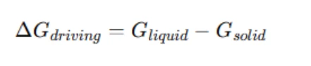
where Gliquid is the Gibbs free energy of the liquid phase at the given composition and temperature, and Gsolid is the Gibbs free energy of the corresponding solid phase at equilibrium.
Step 2: Setting Up the MATLAB Code
Now that we understand the equations involved, we can set up a MATLAB script to automate the calculations. The first step is to define the given thermodynamic data in MATLAB and create functions to compute the Gibbs free energy values for different phases.
% Define temperature
T = 436; % in Kelvin

% Define Gibbs free energy equations
G_Pb_fcc_bct = @(T) 489 + 3.52 * T;
G_Pb_fcc_liquid = @(T) 4810 - 8.017 * T;
G_Sn_bct_fcc = @(T) 5510 - 8.46 * T;
G_Sn_bct_liquid = @(T) 7179 - 14.216 * T;

% Compute Gibbs free energies at given temperature
G_fcc_bct = G_Pb_fcc_bct(T);
G_fcc_liquid = G_Pb_fcc_liquid(T);
G_bct_fcc = G_Sn_bct_fcc(T);
G_bct_liquid = G_Sn_bct_liquid(T);
This initial setup stores the Gibbs free energy changes for phase transformations at the given temperature. Next, we calculate the driving force for phase transformations.
Step 3: Calculating Driving Force for Solidification
The total driving force for solidification of the liquid phase into the equilibrium solid phases (fcc and bct) is given by:
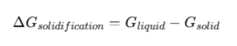
We compute these values for the two given compositions:
% Define equilibrium compositions
X_Sn_liquid = [0.696, 0.9];  % Given compositions
X_Sn_fcc = 0.281;
X_Sn_bct = 0.981;

% Compute driving forces for solidification
G_fcc = G_fcc_liquid - G_fcc_bct;
G_bct = G_bct_liquid - G_bct_fcc;

% Display results
fprintf('Driving force for fcc phase: %.2f J/mol\n', G_fcc);
fprintf('Driving force for bct phase: %.2f J/mol\n', G_bct);
At this point, we have determined how much thermodynamic driving force exists for the liquid phase to solidify into either of the solid phases.
Step 4: Calculating Nucleation Driving Force
For nucleation, we analyze the difference in free energy between the initial liquid phase and the newly forming phase. This determines whether one phase is more likely to nucleate before the other.
% Compute nucleation driving forces
G_nucleation_fcc = G_fcc_liquid - G_fcc_bct;
G_nucleation_bct = G_bct_liquid - G_bct_fcc;

% Display nucleation driving force
fprintf('Nucleation driving force for fcc phase: %.2f J/mol\n', G_nucleation_fcc);
fprintf('Nucleation driving force for bct phase: %.2f J/mol\n', G_nucleation_bct);
If the nucleation driving force is significantly larger for one phase, it is likely to nucleate first. If the values are close, both phases may nucleate simultaneously.
Step 5: Interpreting the Results
After running the MATLAB script, students can compare the driving forces and analyze which phase is more likely to form first. If the nucleation driving force for the fcc phase is much higher than for the bct phase, the fcc phase will nucleate first. If the values are close, both phases may nucleate together. This step involves critically analyzing the computed values and relating them to the physical behavior of the material.
To provide further insights, students can visualize the phase transformation process using MATLAB plots.
% Plot nucleation driving forces
composition = [X_Sn_fcc, X_Sn_bct];
driving_force = [G_nucleation_fcc, G_nucleation_bct];

figure;
bar(composition, driving_force);
xlabel('Composition (X_{Sn})');
ylabel('Driving Force for Nucleation (J/mol)');
title('Nucleation Driving Force for Pb-Sn System');
This visualization helps students understand the trends in nucleation driving forces and how composition affects phase transformations.
Step 6: Extending the Approach to Other Problems
While this blog focuses on a Pb-Sn alloy system, the approach can be generalized to other alloy systems and phase transformation problems. Students can modify the MATLAB script to analyze different materials by changing the given thermodynamic data. Key takeaways include:
- Understanding the problem and identifying relevant equations.
- Writing MATLAB functions to compute Gibbs free energies.
- Calculating driving forces for phase transitions and nucleation.
- Analyzing results through numerical values and visualizations.
This systematic approach equips students with the skills to solve similar MATLAB assignments efficiently. By following this guide, students can develop a deeper understanding of thermodynamics and phase transformations while gaining hands-on MATLAB experience.
Conclusion
Solving MATLAB assignments related to phase transformations and thermodynamics requires a structured approach that combines theoretical understanding with computational analysis. This blog has provided a step-by-step guide to tackling such assignments by defining the problem, setting up Gibbs free energy equations, computing driving forces for solidification and nucleation, and interpreting results. By implementing these steps in MATLAB, students can analyze complex phase transformation problems efficiently.
Beyond the specific Pb-Sn alloy system discussed, this methodology can be applied to a wide range of material science problems. Understanding how to manipulate Gibbs free energy equations and calculate phase equilibria is crucial for students working on thermodynamics, metallurgy, and materials engineering assignments. Using MATLAB for these calculations not only simplifies the computational workload but also allows for visualization and deeper insights into phase stability and transformation mechanisms.
Students are encouraged to extend this approach to other systems by modifying the thermodynamic data and exploring different temperature conditions. Mastering these techniques will enhance their problem-solving skills and prepare them for more advanced applications in material science research and industry.