How to Solve Complex MATLAB Assignment on Power System Modeling

MATLAB is an essential tool in engineering, particularly in power systems, control engineering, and electrical engineering assignments. For students tasked with complex assignments like modeling power systems, such as inverters and filters, MATLAB offers powerful capabilities for handling state-space models, transformations, and simulations. In this blog post, we will guide you step-by-step through how to solve your Power System Modeling assignment using MATLAB, including building state-space representations, applying control techniques, and using MATLAB for simulation. Whether your assignment relates to inverters, filters, or more complex energy systems, this guide will provide a framework to complete your MATLAB assignment with confidence.
Step 1: Understanding the Assignment Scope

In a typical MATLAB assignment that deals with power systems like the one described in the introduction, the goal is to create a model that represents the dynamics of various system components. For example, in an inverter model, the task may involve regulating real and reactive power through current control. Such assignments generally require constructing models in state-space form, simulating system behavior, and performing validation.
For starters, make sure to carefully read the assignment prompt and identify key variables, including power references, voltage, current, system components like filters, inverters, and phase-locked loops (PLLs). Understanding the variables and their relationships is the first step towards modeling them correctly in MATLAB.
Step 2: Building the State-Space Model
One of the most critical steps in these assignments is constructing the state-space model. This model describes how the system’s states evolve over time and how different variables interact within the system.
2.1 What is State-Space Modeling?
State-space modeling is a mathematical framework for modeling dynamic systems. In MATLAB, you will often work with systems that have multiple inputs and outputs, each of which can be represented by vectors. The general state-space representation is given as:
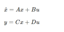
Where:
- x˙ is the state vector derivative (i.e., the rate of change of the states),
- A is the system matrix that describes the system dynamics,
- B is the input matrix that describes how inputs affect the states,
- u is the input vector,
- C is the output matrix that determines how the states are mapped to outputs,
- D is the feedthrough matrix, representing direct interactions between inputs and outputs.
The state-space model is useful for solving differential equations and representing systems that are linear or can be linearized for the purposes of analysis. For your assignment, constructing a state-space model of the inverter system described in the prompt will allow you to simulate its behavior and validate the control system’s performance.
2.2 Subsystems and State-Space Representation
The inverter system described includes various subsystems such as:
- dq-to-abc transformation: This subsystem converts the rotating frame variables into three-phase abc system variables.
- Current controllers: This subsystem ensures that the output current matches the desired reference.
- LC filter: This subsystem models the filtering elements used to reduce high-frequency ripple in the output current.
Each of these subsystems can be modeled using state-space equations. For example, the dq-to-abc transformation can be written as a matrix equation, where the angle of rotation is an input variable. The current controller can be modeled as a feedback system, adjusting the control signals to regulate the current in the inverter output.
In MATLAB, you will need to break down each subsystem and represent it as a state-space equation. For the inverter, start with the voltage and current relationships, and then proceed to incorporate the effects of the PLL and the LC filter.
Step 3: Implementing the Inverter Model in MATLAB
Once you have the individual state-space representations, the next step is to combine them into a complete model of the system. The combined state-space representation for the entire system can be written as:
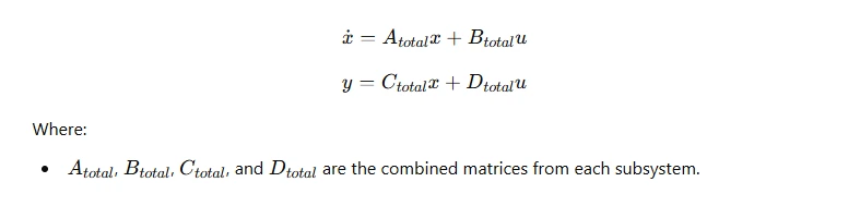
You can now create these matrices in MATLAB using arrays. For example:
A_total = [A_dq_to_abc, A_current_controller, A_LC_filter];
B_total = [B_dq_to_abc, B_current_controller, B_LC_filter];
C_total = [C_dq_to_abc, C_current_controller, C_LC_filter];
D_total = [D_dq_to_abc, D_current_controller, D_LC_filter];
This concatenation of matrices results in a system that can be simulated for different input parameters. The input vector u would typically consist of the voltage references and current references, while the output vector y includes the output currents and possibly the DC link current.
Step 4: Solving the State-Space Model
With the state-space model constructed, the next step is to solve it. In MATLAB, you can solve the system of differential equations using numerical solvers such as ode45, which is commonly used for solving ordinary differential equations.
Here's an example of how you might solve the system:
% Define the state-space system
sys = ss(A_total, B_total, C_total, D_total);

% Solve the differential equation
[t, x] = ode45(@(t, x) A_total*x + B_total*u, [0 T], x0);
Where:
- t is the time vector,
- x is the state vector over time,
- x0 is the initial state vector,
- T is the simulation end time,
- u is the input vector.
Step 5: Validating the Model
After solving the state-space model, the next crucial step is validation. The goal of this step is to verify that your model behaves as expected and compares well with known results or other simulation tools, such as Simulink.
5.1 Comparing with Simulink or Other Tools
In the case of power system simulations, you may have access to a tool like Simulink, which provides a component-based simulation environment. You can compare the results from your MATLAB state-space model with the results from a Simulink model.
For example, you can plot the output currents from both MATLAB and Simulink and check if the waveforms match. MATLAB also allows you to plot the phase currents, output currents, and other key variables, helping you ensure that the state-space model produces realistic results.
figure;
subplot(2, 1, 1);
plot(t, x(:, 1)); % Plot for output current 1
xlabel('Time (s)');
ylabel('Current (A)');
title('Output Current - MATLAB');

subplot(2, 1, 2);
plot(t_simulink, x_simulink(:, 1)); % Plot for output current 1 (Simulink)
xlabel('Time (s)');
ylabel('Current (A)');
title('Output Current - Simulink');
5.2 Checking Performance with Step Responses
Another effective way to validate your model is to test its performance with step responses. By applying step changes to the power reference and observing the system’s response, you can assess the dynamic behavior of the system and make sure that it follows the expected trends.
In MATLAB, you can use the step function to plot the step response:
step(sys);
This function provides a quick way to visualize how the system reacts to changes in inputs over time, allowing you to confirm that your system is stable and behaves as expected.
Step 6: Fine-Tuning the Model
In power system modeling, it’s often necessary to refine and adjust your model to improve accuracy. This could involve adjusting the filter design parameters, adding nonlinear elements like saturation, or improving the resolution of the simulation.
6.1 Handling Nonlinearities
If your system includes nonlinearities, such as saturation effects in the inverter output, you can introduce them into your MATLAB model by using conditional statements within your simulation loop:
if output_voltage > max_voltage
    output_voltage = max_voltage;
elseif output_voltage < min_voltage
    output_voltage = min_voltage;
end
This simple saturation model ensures that the system’s voltage does not exceed predefined limits, which is a common feature in power electronics.
6.2 Optimization of Parameters
Finally, you may need to optimize your model’s parameters, such as filter components or control gains. MATLAB’s optimization toolbox provides several methods to adjust parameters based on performance criteria, such as minimizing error or optimizing system response.
opt_params = fmincon(@(params) objective_function(params), initial_params);
Where objective_function defines the performance criteria (e.g., minimizing error or maximizing efficiency), and fmincon finds the optimal set of parameters.
Step 7: Finalizing Your MATLAB Assignment
Once the model has been validated, refined, and optimized, it’s time to compile the results and present them in a clear and concise manner. Ensure that your assignment report includes:
- A brief explanation of the system being modeled,
- The state-space representation and equations,
- The simulation setup and solver methods used,
- Validation results comparing MATLAB with other tools (e.g., Simulink),
- A discussion on the performance of the system under various conditions,
- Any challenges encountered and how they were addressed.
Also, make sure to document your code properly with comments explaining each part of the process.
Conclusion
Solving complex MATLAB assignments in power systems and control engineering can be a daunting task, but breaking the process down into manageable steps makes it much more approachable. By understanding the system dynamics, constructing a state-space model, implementing it in MATLAB, and validating the results, you can tackle assignments with confidence. Whether you're working on inverter modeling, filter design, or any similar power systems assignment, following these steps will guide you toward producing an accurate and effective solution.