How to Solve MATLAB Assignments on Motion Analysis and Trajectory Plotting

MATLAB is widely used in engineering, physics, biomechanics, and other scientific fields for data analysis, visualization, and numerical computations. Many assignments require students to analyze motion data, including marker trajectories, velocity, and joint angles. Understanding how to process and visualize this data is essential for solving such tasks efficiently. This blog outlines a step-by-step approach on how to solve your matlab assignment related to motion analysis and trajectory plotting. It covers key techniques such as reading data from external files, defining variables, and plotting 3D trajectories to visualize motion. Additionally, it explains how to compute velocity, detect peaks in movement using MATLAB’s findpeaks function, and analyze phase diagrams to understand motion patterns.
Further, the guide provides methods to calculate distances between body markers using vector norms and standard coordinate-based formulas. Finally, it explores how to determine joint angles using the dot product, which is crucial in biomechanics and robotics applications. Although this guide follows a specific example, the concepts and techniques presented can be applied to a variety of assignments in MATLAB. By mastering these skills, students can confidently analyze motion data, interpret results, and improve their problem-solving abilities in computational modeling.

Step 1: Reading and Understanding the Data File
Most motion analysis assignments require reading data from an external file, such as an Excel spreadsheet. MATLAB provides built-in functions like readtable, xlsread, or readmatrix to handle such tasks.
How to Read Data Using readtable
The readtable function is widely used for importing data stored in spreadsheet format. This function reads the data into a table format, making it easy to reference variables by their column names.
% Load the data from an Excel file
data = readtable('trial1.xlsx');

% Display the first few rows of the table
head(data)
Understanding the Data Structure
After loading the data, check the structure using head(data), size(data), or summary(data). This will help identify which columns correspond to marker positions (X, Y, Z coordinates) and time.
Step 2: Defining Variables for Analysis
Once the data is loaded, define the key variables needed for the analysis. These typically include:
- Time Variable: Extract the time column.
- Marker Positions: Extract the X, Y, and Z coordinates of key markers like the shoulder, elbow, and hand.
% Define time variable
time = data.Time;

% Extract X, Y, Z coordinates for relevant markers
shoulder_x = data.Shoulder_X;
shoulder_y = data.Shoulder_Y;
shoulder_z = data.Shoulder_Z;

elbow_x = data.Elbow_X;
elbow_y = data.Elbow_Y;
elbow_z = data.Elbow_Z;

hand_x = data.Hand_X;
hand_y = data.Hand_Y;
hand_z = data.Hand_Z;
Defining variables this way allows for easier manipulation and visualization in later steps.
Step 3: Plotting 3D Trajectories
3D trajectory plots provide insights into the motion of different markers over time.
Using plot3 to Visualize Motion in 3D
The plot3 function in MATLAB is useful for plotting trajectories in three dimensions.
figure;
plot3(hand_x, hand_y, hand_z, 'r', 'LineWidth', 2);
hold on;
plot3(elbow_x, elbow_y, elbow_z, 'g', 'LineWidth', 2);
plot3(shoulder_x, shoulder_y, shoulder_z, 'b', 'LineWidth', 2);
grid on;
xlabel('X-axis');
ylabel('Y-axis');
zlabel('Z-axis');
title('3D Trajectory of Arm Markers');
legend('Hand', 'Elbow', 'Shoulder');
This plot will help visualize how the arm moves in space over time.
Step 4: Creating a Stick Figure of the Arm
A stick figure representation is useful for understanding the connectivity of different joints.
Drawing Lines Between Joints
To create a stick figure, plot lines connecting the markers at a specific time frame.
t_index = 1; % Select the first time step (Time=0)
figure;
plot3([shoulder_x(t_index), elbow_x(t_index), hand_x(t_index)], ...
      [shoulder_y(t_index), elbow_y(t_index), hand_y(t_index)], ...
      [shoulder_z(t_index), elbow_z(t_index), hand_z(t_index)], 'ko-', 'LineWidth', 3);

grid on;
xlabel('X-axis');
ylabel('Y-axis');
zlabel('Z-axis');
title('Stick Figure of the Arm at Time = 0');
This plot represents the structure of the arm at the initial time step.
Step 5: Plotting X, Y, and Z Coordinates Over Time
To analyze the motion of the hand marker, plot its X, Y, and Z coordinates over time.
figure;
subplot(3,1,1);
plot(time, hand_x, 'r', 'LineWidth', 2);
xlabel('Time (s)'); ylabel('X Coordinate');
title('Hand X Coordinate Over Time');

subplot(3,1,2);
plot(time, hand_y, 'g', 'LineWidth', 2);
xlabel('Time (s)'); ylabel('Y Coordinate');
title('Hand Y Coordinate Over Time');

subplot(3,1,3);
plot(time, hand_z, 'b', 'LineWidth', 2);
xlabel('Time (s)'); ylabel('Z Coordinate');
title('Hand Z Coordinate Over Time');
This visualization helps understand how the hand moves in each dimension separately.
Step 6: Calculating and Plotting Hand Velocity
Velocity can be computed by differentiating the position data.
hand_velocity_x = diff(hand_x) ./ diff(time);

% Adjust time array to match velocity length
time_velocity = time(2:end);

figure;
plot(time_velocity, hand_velocity_x, 'r', 'LineWidth', 2);
xlabel('Time (s)');
ylabel('Velocity (m/s)');
title('Hand Velocity Along X Axis');
Step 7: Identifying Peaks in Velocity
Using findpeaks, we can detect the highest velocity points.
[pks, locs] = findpeaks(hand_velocity_x, time_velocity, 'MinPeakHeight', 0.1);

figure;
plot(time_velocity, hand_velocity_x, 'b', 'LineWidth', 2);
hold on;
plot(locs, pks, 'ro', 'MarkerSize', 8, 'MarkerFaceColor', 'r');
xlabel('Time (s)');
ylabel('Velocity (m/s)');
title('Velocity Peaks');
legend('Velocity', 'Peaks');
Step 8: Plotting a Phase Diagram
A phase diagram plots velocity against position.
figure;
plot(hand_x(2:end), hand_velocity_x, 'k', 'LineWidth', 2);
xlabel('Position (X)');
ylabel('Velocity (X)');
title('Phase Diagram: Hand Motion Along X Axis');
grid on;
This graph provides insight into dynamic behavior.
Step 9: Calculating Distance Between Shoulder and Hand
The distance between two points in 3D space is computed using:
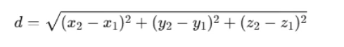
distance_shoulder_hand = sqrt((hand_x - shoulder_x).^2 + (hand_y - shoulder_y).^2 + (hand_z - shoulder_z).^2);

figure;
plot(time, distance_shoulder_hand, 'm', 'LineWidth', 2);
xlabel('Time (s)');
ylabel('Distance (m)');
title('Distance Between Shoulder and Hand');
Using vecnorm:
distance_norm = vecnorm([hand_x - shoulder_x, hand_y - shoulder_y, hand_z - shoulder_z], 2, 2);
Step 10: Calculating and Plotting Elbow Angle
Using the dot product, we can calculate the elbow angle.
v1 = [elbow_x - shoulder_x, elbow_y - shoulder_y, elbow_z - shoulder_z];
v2 = [hand_x - elbow_x, hand_y - elbow_y, hand_z - elbow_z];

dot_product = sum(v1 .* v2, 2);
magnitude_v1 = sqrt(sum(v1.^2, 2));
magnitude_v2 = sqrt(sum(v2.^2, 2));

elbow_angle = acosd(dot_product ./ (magnitude_v1 .* magnitude_v2));

figure;
plot(time, elbow_angle, 'g', 'LineWidth', 2);
xlabel('Time (s)');
ylabel('Elbow Angle (degrees)');
title('Elbow Angle Over Time');
Conclusion
By following these steps, students can systematically analyze motion data in MATLAB, making it easier to handle assignments related to biomechanics, robotics, and motion tracking. The key to solving such problems lies in understanding how to read and manipulate data, define relevant variables, and visualize motion using 2D and 3D plots. Starting with reading the dataset using readtable, students can extract necessary coordinates for different markers like the shoulder, elbow, and hand. Plotting 3D trajectories helps visualize motion patterns, while stick figure representations provide a simplified skeletal structure. Analyzing X, Y, and Z coordinates over time allows for detailed motion tracking. Velocity calculations using numerical differentiation help determine movement dynamics, and findpeaks aids in identifying significant velocity changes. Phase diagrams offer insight into position-velocity relationships. Calculating distances between markers, using both standard formulas and MATLAB’s norm function, ensures accurate measurement. Finally, computing joint angles using the dot product provides valuable kinematic analysis. By mastering these techniques, students can efficiently work through similar MATLAB assignments, whether in biomechanics, robotics, or other motion analysis fields. Understanding these fundamentals will improve their ability to analyze movement and interpret real-world motion data effectively.