Efficient Ways to Solve MATLAB Assignments Involving Heat Transfer Simulations

Heat transfer problems frequently arise in engineering, especially in material processing and thermal system design. A common challenge in MATLAB assignments involves simulating the cooling process of a metal plate cast in a sand mold using the explicit control volume-based finite difference method (CV-FDM) in one dimension with Cartesian coordinates. Understanding how to approach such assignments is essential, as the techniques used in this problem apply to various heat transfer simulations.
In this type of assignment, students must develop a numerical solver that iterates forward in time to compute temperature changes at discrete nodes. The cooling process is modeled as a one-dimensional system, considering heat transfer between the casting, mold, and surrounding atmosphere. The explicit CV-FDM method discretizes the heat conduction equation to update temperatures at each node based on its neighbors. Ensuring numerical stability requires careful selection of the time step, following the Courant-Friedrichs-Lewy (CFL) condition.

This blog will provide a structured approach on how to solve your MATLAB assignment, covering key aspects such as boundary conditions, solver implementation, stability criteria, and result validation. By following these steps, students can gain a deeper understanding of computational heat transfer and develop strong problem-solving skills for engineering applications.
Understanding the Problem and the Given Code Structure
Before implementing a solution, students should begin by carefully analyzing the problem statement and the MATLAB code provided. Typically, assignments of this nature include an unfinished script that sets up the computational domain, boundary conditions, and initial temperature distribution. The goal is to develop a numerical solver that calculates temperature evolution over time using finite difference approximations.
The simulation considers only one side of the casting due to symmetry. The heat transfer problem is modeled as a one-dimensional system where temperatures at discrete nodes evolve over time. Nodes outside the sand mold represent the surrounding atmosphere and are assigned a high specific heat capacity to simulate an infinite thermal mass. The key challenge is to iteratively compute temperature changes at each node while ensuring stability and accuracy.
Students should begin by running the provided code and stepping through it line by line. This can be done by setting breakpoints and using MATLAB's debugging tools, such as the F10 key to execute code incrementally. Observing variable values in the workspace allows students to understand the data structures used in the program and identify where modifications are needed.
Setting Up the Explicit CV-FDM Solver
The explicit finite difference method is a time-marching scheme that calculates future temperatures based on known values from the previous time step. The governing equation for heat transfer in a one-dimensional system is derived from the heat conduction equation:
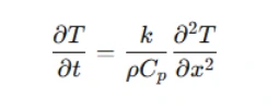
where T is the temperature, k is the thermal conductivity, ρ is the density, and Cp is the specific heat capacity. Discretizing this equation using the control volume method results in an explicit update formula for each node in the computational mesh.
In MATLAB, the solver must iterate through time and update temperatures at each node using finite difference approximations. The temperature at each interior node is updated based on the temperatures of its neighboring nodes. The discretized equation takes the form:
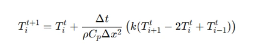
where Δt is the time step and Δx is the spatial step. This equation must be implemented as a loop in MATLAB, ensuring that temperatures are updated correctly at each iteration.
Choosing an Appropriate Time Step
One of the most important considerations in explicit finite difference methods is selecting a time step that ensures numerical stability. The stability criterion for the explicit method is given by the Courant-Friedrichs-Lewy (CFL) condition:
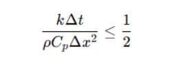
If the time step is too large, the solution may become unstable and produce non-physical oscillations. To avoid this, students should compute the maximum allowable time step based on material properties and mesh resolution before running the simulation.
Implementing Boundary Conditions
Boundary conditions play a crucial role in determining the accuracy of the simulation. In this assignment, two key boundary conditions must be enforced:
- Insulated Boundaries: Nodes at the edges of the domain (fictive nodes 1 and 16) should not exchange heat with their surroundings. This is achieved by setting the temperature gradient to zero, ensuring that no heat flows across these boundaries.
- Heat Exchange Between Casting and Mould: The interface between the casting and the sand mold must be handled carefully to account for heat transfer between materials with different thermal properties. The heat flux at this interface should be continuous, meaning that conduction from the casting must equal conduction into the mold.
In MATLAB, these boundary conditions are implemented by modifying the update equations for the first and last physical nodes. Instead of using standard finite difference formulas, the temperature changes at boundary nodes must be adjusted to reflect the absence of heat flux or material property discontinuities.
Running the Simulation and Checking for Convergence
Once the solver is implemented, the next step is to run the simulation and ensure that it terminates correctly. The stopping condition for this assignment is when the temperature at the node closest to the center of the plate drops below a specified threshold (e.g., 1050°C).
Students should modify the while-loop condition so that the program continues running until this criterion is met. If the simulation does not stop, it often indicates that the end condition is never satisfied due to incorrect logic or numerical errors. In such cases, manually interrupting execution with CTRL+C and debugging the code can help identify the issue.
Validating Results and Ensuring Energy Conservation
After running the simulation, students must analyze the results to ensure that the computed temperatures are reasonable. Several validation steps should be performed:
Plotting Temperature Profiles: Generating a plot of the temperature distribution at different time steps helps visualize the cooling process. If the results are physically meaningful, the temperature should decrease smoothly over time, with heat flowing from the casting to the mold and surrounding air.
Checking Energy Conservation: If no internal heat generation occurs and boundaries are insulated, the total heat content of the system should remain constant. Students can verify this by computing the total thermal energy in the system at each time step using the formula:
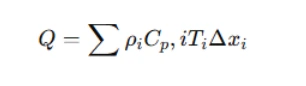
Plotting the evolution of heat content over time should show minimal variation, confirming that energy is conserved throughout the simulation.
Tracking the Center Node Temperature: Since the assignment requires monitoring the temperature at the node closest to the plate’s center, students should plot its evolution over time. The curve should show a steady decrease in temperature, eventually reaching the stopping criterion. If the curve exhibits unexpected jumps or irregularities, it may indicate an instability in the solver that needs to be addressed.
Documenting and Submitting the Assignment
Finally, students should prepare a detailed report summarizing their findings and explaining their MATLAB implementation. Key elements to include are:
- A description of the problem and numerical method used
- An explanation of boundary conditions and solver implementation
- A discussion of numerical stability and time step selection
- Plots illustrating temperature evolution, heat conservation, and node behavior
- Conclusions on the accuracy and reliability of the results
The MATLAB script file should also be well-documented with comments explaining each section of the code. Properly labeling axes in plots and adding a title with the student’s name ensures clarity and completeness in the submission.
Conclusion
Understanding MATLAB assignments related to heat transfer simulations using the control volume-based finite difference method (CV-FDM) requires a structured approach. Students must begin by analyzing the given problem, ensuring they understand the numerical method and provided MATLAB code. The key to solving such problems lies in implementing an explicit finite difference solver that iteratively updates temperatures at each node while maintaining numerical stability. Selecting an appropriate time step is crucial to avoid instability, and applying correct boundary conditions, such as insulation and heat exchange at interfaces, ensures accurate results. Once the solver is implemented, students should validate their results by plotting temperature profiles, checking energy conservation, and tracking the cooling behavior of key nodes. If the simulation does not behave as expected, debugging techniques such as stepping through code and adjusting parameters can help refine the solution.
By mastering these techniques, students not only gain confidence in solving coursework assignments but also develop essential skills for real-world applications in thermal engineering and numerical modeling. Computational heat transfer is a critical area in engineering, and with careful attention to detail, students can build a strong foundation in numerical simulations using MATLAB.