Data Analysis Using MATLAB
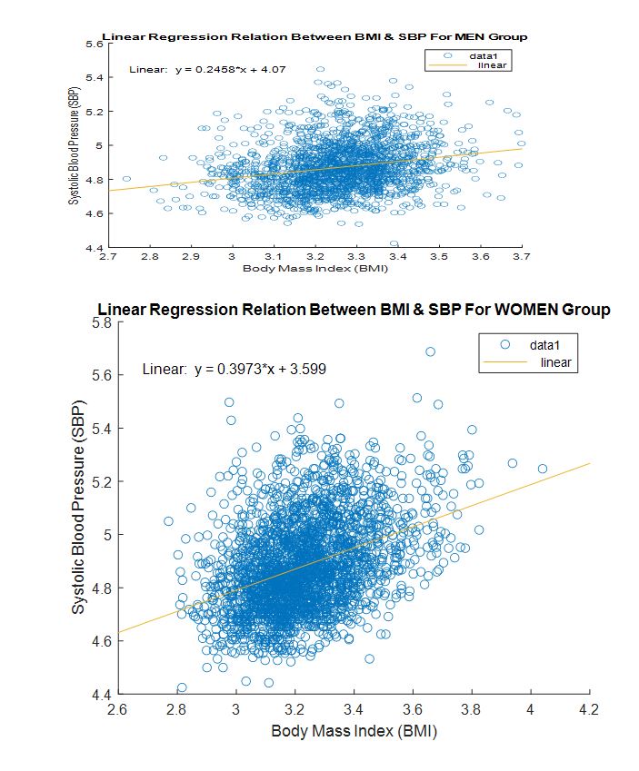
Linear Regression
| Sex | Number of subjects ni | β0 | β 1 |
| Men | 1194 | 4.07 | 0.2458 |
| Women | 2490 | 3.599 | 0.3973 |
Using the Function ‘coefCI’to Find a 95% CI on β 1 Values
Table 2. Confidence intervals on β 1 values
| Sex | Lower Bound | Upper Bound |
| Men | 0.1993 | 0.2923 |
| Women | 0.3599 | 0.4347 |
Multiple Regression Model
| Model | β 1 | P-value for β 1 | R2 |
| a | 1.7885 | 0.0000 | 0.1076 |
| b | 1.0297 | 0.0000 | 0.1588 |
| c | 0.1004 | 0.0000 | 0.0400 |
| Estimate | SE | tStat | pValue | |
| Intercept | 40.8364 | 0.2407 | 460.6981 | 0.0000 |
| BMI | 1.4945 | |||
| Age | 0.8749 | |||
| SCL | 0.0412 |
7. Comment on the significance of regression for each of the three regressors.
Answer: After using multiple regression model, BMI has the more effect on the SBP compared to Age and SCL.
8. Predict the value of SBP for an individual with a BMI of 33, an age of 55 years, and a cholesterol level of 288 mg/dL. Include a 95% prediction interval.
Answer: The equation after multiple linear regression is came out to be: SBP=40.8364+1.4945xBMI+0.8749xAge+0.0412xSCL. After putting the values, we get SBP=150.14.
Extra Credit: Create a new multiple regression model to predict SBP using the Framingham data set. All regressors must be significant and your adjusted R2must be above 0.25 to get credit. Show the results of your model in a table similar to table 4.
Analysis 1 Solution
clc
clear all
close all
%%%%%%%%% Import Framingham data
data=readtable('framingham1.xls'); %%%% reading data from excelsheet
data=data{:,:}; %%%% converting table into matrix form
data2=data(1:4434,:); %%%% selecting data for Period 1 only
data3=sortrows(data2,2); %%%% sorting data based on gender
%%
%%%%%%% For men
BMI_men=log(data3(1:1944,9)); %%%% loading BMI data for men (independent variable)
SBP_men=log(data3(1:1944,5)); %%%% loading SBP data for men (dependent variable)
X=[ones(size(BMI_men)) BMI_men]; %%%% making X matrix for the linear regression model
Y=SBP_men;
[b_men,bint_men]=regress(Y,X) %%%% applying linear regression model to find coefficients and CIs
%%%%% using model to predict SBP values for men
x_men=33;
y_men=0.2458*x_men+4.07
%%
%%%%%%% For WOMEN
BMI_women=log(data3(1945:end,9)); %%%% loading BMI data for women (independent variable)
SBP_women=log(data3(1945:end,5)); %%%% loading SBP data for women (dependent variable)
X=[ones(size(BMI_women)) BMI_women]; %%%% making X matrix for the linear regression model
Y=SBP_women;
[b_women,bint_women]=regress(Y,X) %%%% applying linear regression model to find coefficients and CIs
%%%%% using model to predict SBP values for women
x_women=33;
y_women=0.3973*x_women+3.599
%%
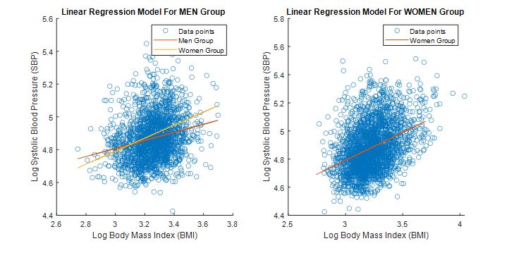
%%%%%% ploting
subplot(1,2,1)
yCalc1_men1=0.2458.*BMI_men+4.07;
yCalc1_women1=0.3973.*BMI_men+3.599;
scatter(BMI_men,SBP_men)
hold on
plot(BMI_men,yCalc1_men1)
hold on
plot(BMI_men,yCalc1_women1)
xlabel('Log Body Mass Index (BMI)')
ylabel('Log Systolic Blood Pressure (SBP)')
title('Linear Regression Model For MEN Group')
legend('Data points','MenGroup','Women Group')
subplot(1,2,2)
scatter(BMI_women,SBP_women)
hold on
hold on
plot(BMI_men,yCalc1_women1)
xlabel('Log Body Mass Index (BMI)')
ylabel('Log Systolic Blood Pressure (SBP)')
title('Linear Regression Model For WOMEN Group')
legend('Data points','Women Group')
Analysis 2 Solution
clc
clear all
close all
%%%%%%%%% Import Framingham data
data=readtable('framingham1.xls'); %%%% reading data from excelsheet
data=data{:,:}; %%%% converting table into matrix form
data2=data(1:4434,:); %%%% selecting data for Period 1 only
%%
%%%%%% Model 1: SBP against BMI without separating the data by sex
BMI_1=data2(:,9); %%%% loading BMI data (independent variable)
SBP_1=data2(:,5); %%%% loading SBP data (dependent variable)
X1=[ones(size(BMI_1)) BMI_1]; %%%% making X matrix for the linear regression model
Y1=SBP_1;
[b1,~,~,~,stats_1]=regress(Y1,X1) %%%% applying linear regression model to find coefficients
%%
%%%%%% Model 2: SBP against age
AGE_2=data2(:,4); %%%% loading AGE data (independent variable)
SBP_2=data2(:,5); %%%% loading SBP data (dependent variable)
X2=[ones(size(AGE_2)) AGE_2]; %%%% making X matrix for the linear regression model
Y2=SBP_2;
[b2,~,~,~,stats_2]=regress(Y2,X2) %%%% applying linear regression model to find coefficients
%%
%%%%%% Model 3: SBP against serum cholesterol
TOTCHOL_3=data2(:,3); %%%% loading Serum Total Cholesterol data (independent variable)
SBP_3=data2(:,5); %%%% loading SBP data (dependent variable)
X3=[ones(size(TOTCHOL_3)) TOTCHOL_3]; %%%% making X matrix for the linear regression model
Y3=SBP_3;
[b3,~,~,~,stats_3]=regress(Y3,X3) %%%% applying linear regression model to find coefficients
%%
%%%%%% Multivariate Linear Regression Model
%%%%%% Multivariate Model: SBP against serum cholesterol
X1=data2(:,9); %%%% loading BMI data (independent variable)
X2=data2(:,4); %%%% loading AGE data (independent variable)
X3=data2(:,3); %%%% loading Serum Total Cholesterol data (independent variable)
SBP=data2(:,5); %%%% loading SBP data (dependent variable)
Y=SBP;
X=[ones(size(X1)) X1 X2 X3]; %%%% making X matrix for the linear regression model
[beta,~,~,~,stat]=regress(Y,X) %%%% applying linear regression model