How to Solve Complex MATLAB Assignments on Numerical Methods

Dr. Raymond Caldwell

Australia

MATLAB

Dr. Raymond Caldwell, with over 12 years of experience in MATLAB numerical methods, earned his Ph.D. in Computational Mathematics from the University of Wollongong, Australia.

Hire Me To Do Your MATLAB Assignment

Before diving into the solution process, it is crucial to comprehend the nature of the problem at hand. In most mathematical modeling problems, like solving the second-order hyperbolic equation:

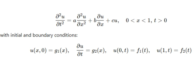
It is important to first identify the problem type. Here, we are dealing with a second-order PDE. The boundary and initial conditions give us further information about how the solution evolves. By identifying these elements early on, you can decide which numerical method to apply.

2. Decoding the Difference Scheme

For the second-order hyperbolic equation, the solution is given by a difference scheme, which is essentially a discretization of the PDE. The equation involves multiple terms, and understanding these terms is crucial:

Understanding this equation is key. The coefficients β1, β2, β3, along with the terms λ, k, h, θ, represent various parameters related to the problem’s discretization. They help in calculating the next steps based on the current solution.

The discretization in MATLAB will involve setting up grids for both time and space. Each grid point will represent a value for u at a specific time and space location. Using MATLAB's built-in functions for finite difference schemes, students can apply the equations iteratively to solve for the solution at each grid point.

How to Approach

1. Set up the grid: Choose values for the space step Δx and time step Δt. Define the spatial domain [0,1] and the time domain t > 0, and divide them into small intervals.
2. Initial and boundary conditions: Implement the provided initial and boundary conditions in MATLAB. These will serve as the starting points for your iterative solution.
3. Difference equation implementation: Use the difference equation to iteratively solve for un+1m at each grid point. This is the core step where MATLAB’s array manipulation capabilities are most useful.

3. Stability and Consistency of the Numerical Scheme

For numerical schemes like the one above, analyzing the stability and consistency is essential. Stability ensures that small errors in the numerical solution do not grow uncontrollably, and consistency ensures that the numerical method approximates the true solution as the grid spacing tends to zero.

Local Truncation Error

In the context of the given second-order hyperbolic equation, the local truncation error represents the error introduced by the finite difference approximation at each time step. The goal is to minimize this error as much as possible.

To calculate the local truncation error for the given scheme, you need to perform a series of steps:

1. Calculate the exact solution of the equation (if possible) or use an analytical method to derive the theoretical error.
2. Compare the numerical solution obtained using the difference scheme with the exact solution. The difference between the two will provide you with an estimate of the truncation error.

Stability Criterion

The stability criterion can be obtained by performing a von Neumann stability analysis. This involves substituting a trial solution into the difference equation and examining the growth of errors over time. Stability ensures that the numerical method does not produce exponentially growing errors for any perturbation in the solution.

4. Applying Numerical Methods to Other Problems

The methods outlined above can be applied to a range of problems, from simple diffusion equations to more complex fluid mechanics problems.

Example 1: Diffusion-Reaction Problem

Consider a diffusion-reaction problem, such as:

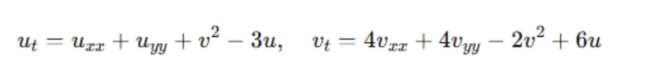
This problem involves both diffusion and reaction terms for the variables u and v. Similar to the hyperbolic equation, the key is to discretize both space and time.

1. Discretization of PDEs: Use finite differences for the second-order spatial derivatives, and forward Euler or Crank-Nicolson schemes for the time derivative.
2. Boundary and initial conditions: Implement the boundary conditions (e.g., u = v = 1 at x = 0, 1) and the initial conditions u(x, y, 0) = v(x, y, 0) = 1.
3. Numerical solution: Solve the equations iteratively using MATLAB. Plot the solution at different time steps to analyze the behavior of u and v.

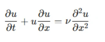
Example 2: Burgers' Equation

Burgers’ equation is another classic problem in fluid mechanics:

1. Explicit Methods: Apply explicit finite difference methods such as forward Euler for time and central differences for space.
2. Boundary and initial conditions: Use the given initial condition u(x, 0) = −sin(πx) and boundary conditions u(−1, t) = u(1, t) = 0.
3. Numerical solution: Solve the equation for different values of ν and plot the solution over time.

5. Solving the Wave Equation

The wave equation:

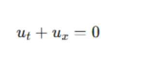
is a simple hyperbolic equation that models wave propagation. For such equations, the focus is on wave speed and group speed. The wave is represented as a sine wave, and the goal is to track its propagation over time.

1. Finite difference schemes: Implement different schemes, such as leapfrog, Crank-Nicolson, or fourth-order leapfrog. Each scheme will have a different dispersion relation, wave speed, and group speed.
2. Numerical solution: Use MATLAB to simulate the wave propagation. For each scheme, calculate the wave speed and group speed using the dispersion relation. This will give you insight into how the numerical scheme handles wave propagation.

6. Practical Tips for Solving MATLAB Assignments

Here are some practical tips to help you tackle similar MATLAB assignments:

1. Understand the problem first: Before jumping into MATLAB, ensure that you understand the physical or mathematical context of the problem. This will help you decide on the best approach for discretization and numerical methods.
2. Break down the problem: Decompose the problem into smaller, manageable parts. Solve the initial and boundary conditions, discretize the PDE, and then proceed with the numerical method.
3. Use MATLAB functions effectively: MATLAB has a wide range of functions for solving PDEs and performing numerical computations. Learn how to use built-in functions like diff for derivatives and ode45 for solving differential equations.
4. Test your solution: Once you've implemented your numerical method, test it with simple cases for which you know the analytical solution. This will help you identify errors in your implementation.
5. Analyze the results: Plot the solution at different time steps to visualize how the variables evolve. Look for any instability or divergence in the solution, and adjust your numerical method or grid size accordingly.

Conclusion

MATLAB assignments can seem complex, especially when dealing with partial differential equations and numerical schemes. However, by following a structured approach, you can solve these problems efficiently. Break down the problem, discretize the equations, apply the appropriate numerical method, and analyze the results. With practice, you'll become more comfortable handling such assignments and be able to apply the methods to a wide range of problems. If you ever feel stuck, remember that MATLAB has a robust community, and many resources are available online. You can also seek help from MATLAB experts who can guide you through the process and provide the support you need.

By mastering these techniques, you'll be well-equipped to handle similar MATLAB assignments and achieve great results in your studies.