How to Solve Electrical System Assignments Using MATLAB and Simulink

MATLAB and Simulink are widely used software tools in electrical engineering, control systems, and various other fields to solve complex problems. These tools are especially helpful for students dealing with assignments that require system modeling, simulation, and analysis of electrical circuits. Assignments such as solving equations in the Laplace domain, analyzing transfer functions, or simulating system behavior often form the core of many academic tasks. For students, these types of problems can seem challenging at first. However, with the right approach and systematic steps, solving these assignments becomes more manageable and rewarding. This comprehensive guide aims to provide students with the knowledge and methodology to solve their Simulink assignment efficiently, whether you're working on system stability analysis, transient analysis, or electrical circuit behavior.
Step 1: Understanding the Assignment Requirements
The first step in tackling any MATLAB and Simulink assignment is to carefully understand the problem at hand. Often, assignments in electrical engineering and systems analysis ask you to use MATLAB to simulate circuit behaviors, solve system equations, and analyze system performance based on theoretical principles. These tasks may involve:

- Solving system equations in the Laplace domain.
- Determining system stability, such as evaluating damping coefficients and natural frequency.
- Graphing and commenting on the simulated results to assess stability and system behavior.
- Simulating circuits using MATLAB and Simulink and analyzing parameters like rise time, peak time, settling time, and overshoot.
- Using MATLAB’s built-in functions such as step(), bode(), pzmap(), and others to analyze system performance.
- Exporting data and visualizations (such as graphs and charts) for inclusion in assignment reports.
It is important to break the problem into smaller, manageable parts and systematically approach each step. Often, MATLAB will generate code and results in a structured manner, which makes it easier to understand what is happening within the system, but a well-laid-out approach will allow you to work efficiently.
Step 2: Solving System Equations in the Laplace Domain
One common task in these assignments is solving system equations in the Laplace domain. The Laplace transform is an integral transform that converts complex time-domain differential equations into simpler algebraic equations in the s-domain. This approach simplifies solving linear differential equations, especially when analyzing circuit systems and dynamic control processes.
Formulating the Transfer Function
When you are asked to solve equations in the Laplace domain, your first task is to obtain the transfer function of the system. The transfer function describes the system's behavior in the Laplace domain and is typically written in the form of a ratio of polynomials.
For example, if you're working on a circuit consisting of a resistor (R), an inductor (L), and a capacitor (C), you can obtain the transfer function of the circuit by considering the impedance of each element and applying Kirchhoff's laws.
Step-by-Step Example in MATLAB:
- Declare the values for the components in the circuit:
- Define the Laplace variable s using the MATLAB tf command:
- Define the transfer function:
R1 = 50;        % Resistor value in ohms
L1 = 100e-3;    % Inductor value in Henry (100 mH)
C1 = 20e-6;     % Capacitor value in Farads (20 uF)
s = tf('s');
transfer_function = 1 / (R1*C1*s + L1);
Analyzing Stability
Once the transfer function is obtained, the next step is to analyze its stability. In control systems, stability is crucial as it dictates whether the system will reach a steady-state or exhibit oscillatory behavior. Stability can be assessed by looking at the poles and zeros of the transfer function.
The damping coefficient (ζ) and natural frequency (ω_n) are important parameters in determining the stability of the system. You can calculate these from the coefficients of the transfer function. For a second-order system, the damping coefficient can be calculated as:
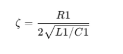
This value helps you determine whether the system is overdamped, critically damped, or underdamped.
You can also use MATLAB’s pole() function to find the poles of the transfer function:
poles = pole(transfer_function);
The poles' locations on the complex plane will give you insights into system behavior. If the poles are on the real axis, the system is overdamped; if the poles are complex, the system is underdamped.
Step 3: Simulating the Circuit in Simulink
Simulink is a graphical environment for modeling, simulating, and analyzing multidomain dynamic systems. For students working on electrical circuits or control systems, Simulink provides an intuitive interface to visualize and simulate circuits.
Building the Circuit Model
In Simulink, you can represent the circuit using blocks such as Resistor, Inductor, Capacitor, and Voltage Source. These blocks can be found in the Simulink library under the Simscape > Foundation > Electrical section.
- Start by dragging the blocks that represent the components of your circuit.
- Connect the blocks appropriately to match the circuit diagram provided in the assignment.
- Use the Scope block to observe the signal output and analyze the system's behavior over time.
Running Simulations and Analyzing Results
After creating the model in Simulink, you can run the simulation to observe the system's time-domain response. The Scope block in Simulink will show you how the system behaves in response to inputs such as step functions, impulse functions, or sinusoidal inputs.
Example: Analyzing a Step Response
You can use the step() function in Simulink or MATLAB to analyze how the system reacts to a step input. In Simulink, simply add a Step block, connect it to your circuit model, and use a Scope to visualize the output.
The resulting graph will show the rise time, peak time, and settling time. These are key performance parameters in control systems.
Using Powergui and FFT for Signal Analysis
Simulink provides the Powergui block, which is useful for analyzing steady-state conditions, RMS (Root Mean Square) values, and peak values. You can use it to gather information about voltage and current signals, especially in power systems.
Additionally, the Fast Fourier Transform (FFT) block can be used to analyze the frequency components of the system’s signals. This will help you identify harmonics and compare the results with standards like IEEE 519 for Total Harmonic Distortion (THD).
Step 4: Analyzing System Response and Performance
After running the simulation, the next task is to analyze the system’s response. You will need to focus on key performance metrics like:
- Rise Time: The time taken for the system's response to go from 10% to 90% of its final value.
- Peak Time: The time taken to reach the highest point in the response.
- Settling Time: The time taken for the response to settle within a certain percentage (usually 2%) of its final value.
- Overshoot: The amount by which the system exceeds its final value before settling.
To calculate these parameters, you can use the MATLAB stepinfo() function:
info = stepinfo(transfer_function);
rise_time = info.RiseTime;
peak_time = info.PeakTime;
settling_time = info.SettlingTime;
These values will help you assess the system’s transient and steady-state behavior.
Step 5: Using MATLAB for Frequency Response Analysis
In many assignments, you'll need to analyze the frequency response of a system. The Bode plot is one of the most common tools used for this purpose. It provides information about the gain and phase of the system as a function of frequency.
Bode Plot
To generate a Bode plot in MATLAB, you can use the bode() function:
bode(transfer_function);
This plot shows the magnitude and phase of the system across a range of frequencies. You can use this to analyze the system's performance at different frequencies and understand its behavior in the frequency domain.
Pole-Zero Plot
A pole-zero plot is another important tool for analyzing the stability of a system. You can use the pzmap() function to visualize the poles and zeros of the transfer function:
pzmap(transfer_function);
This plot helps you identify the stability of the system and its response characteristics.
Other Frequency Domain Tools
You can also use the Nyquist plot, Nichols chart, and Root Locus plots to analyze the system’s stability and behavior at different frequencies. These plots are particularly useful in control systems and electrical circuit analysis.
Step 6: Exporting Data and Final Report
Once you've completed your analysis and obtained all the necessary results, you need to prepare your final report. MATLAB allows you to export your work, including the code and graphs, into an HTML report.
- Use the publish() function to export your MATLAB code and results into an HTML file:
- Save your Simulink model as a .slx file, which you can then attach to your report.
publish('your_script.m');
Make sure to include clear and detailed comments in your code, explaining each step of the process. This not only helps you understand the problem better but also ensures that anyone reviewing your work can follow your thought process.
Step 7: Comparing Results and Drawing Conclusions
Many assignments will ask you to compare your simulation results with theoretical values or textbook examples. This comparison is crucial in understanding how accurately your model represents real-world systems.
- Compare the rise time, settling time, and overshoot from your simulation with the theoretical values.
- Discuss any discrepancies and provide possible explanations, such as numerical approximation errors, simulation model limitations, or assumptions made during the analysis.
Use your findings to draw meaningful conclusions about the system’s behavior and how well it meets the expected performance.
Conclusion
Solving MATLAB and Simulink assignments doesn't have to be overwhelming. By following a structured approach, understanding the fundamental concepts, and using the powerful tools available in MATLAB and Simulink, you can efficiently tackle complex problems in electrical systems and control theory. Whether you are solving equations in the Laplace domain, simulating a circuit in Simulink, or analyzing system performance, the process becomes much more manageable with practice and a clear understanding of the steps involved. This guide has provided you with a systematic approach to solve your MATLAB assignment, helping you develop the skills needed to analyze, simulate, and understand complex electrical systems and control systems.