How to Approach MATLAB Assignments Involving Bottle Rocket Trajectory

Numerical modeling has become an essential skill in engineering education, especially when it comes to solving problems that are too complex for traditional analytical techniques. These problems often appear in university assignments where students are asked to model and simulate real-world systems using computational tools. One of the most popular and educational examples of such systems is the flight of a bottle rocket. While it may appear to be a simple toy at first glance, modeling the dynamics of a bottle rocket in MATLAB requires a deep understanding of physics, numerical methods, and programming.
In this blog, we will explore how to solve your MATLAB assignment involving numerical modeling, particularly those that require solving differential equations to simulate physical systems. Although our example will revolve around the trajectory of a bottle rocket, the techniques and steps discussed here can be easily adapted to other mechanical or aerospace engineering problems.
Understanding the Physics Behind the System

Before diving into code or equations, it is crucial to thoroughly understand the physical behavior of the system you are trying to model. In the case of a bottle rocket, the trajectory can be divided into three distinct phases. The first is the thrust phase, during which water is rapidly expelled from the bottle due to the internal pressure created by compressed air. This generates thrust and propels the rocket upward.
The second phase, often called the post-exhaust or air thrust phase, begins once all the water has been expelled. During this time, any remaining pressurized air inside the bottle continues to expand, adding a smaller amount of thrust until the internal pressure equals atmospheric pressure. Finally, the rocket enters the ballistic phase, where it moves purely under the influence of gravity and air resistance, following a parabolic path until it eventually lands.
Understanding these phases is important because each one involves different forces and behaviors. A comprehensive simulation must account for the varying mass of the rocket as water is expelled, the changing thrust force, the influence of air resistance, and the gravitational force acting on the rocket at all times.
This deep understanding of the physical system is not only the first step in modeling but also one of the most crucial. Without a clear picture of what is happening physically, it becomes difficult to correctly formulate the equations or make reasonable assumptions in the simulation.
Deriving the Governing Equations
Once the physical phenomena are clearly understood, the next step is to convert them into mathematical terms. The equations that govern the motion of the rocket are rooted in Newton’s second law of motion: the net force acting on an object is equal to its mass multiplied by its acceleration. However, applying this law to a rocket is more complex than it first appears because both the mass and the forces acting on the rocket change over time.
During the thrust phase, the bottle rocket experiences a thrust force due to the ejection of water, a drag force caused by air resistance, and a downward gravitational force. The thrust force can be calculated using the equation:
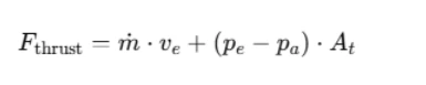
In this equation, m˙ represents the mass flow rate of water exiting the bottle, ve is the exit velocity of the water, pe is the internal pressure of the bottle, pa is the ambient atmospheric pressure, and At is the cross-sectional area of the nozzle through which water is expelled.
The drag force is another key element to consider, and it can be calculated using the formula:
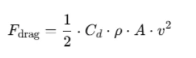
Here, Cd is the drag coefficient, ρ is the density of air, A is the cross-sectional area of the rocket, and v is the velocity of the rocket.
Together, these forces influence the rocket’s motion, and they must be incorporated into the equations that define acceleration in both the horizontal and vertical directions. Because the rocket's mass changes as water is expelled and because the thrust phase transitions to the ballistic phase, the equations are time-dependent and non-linear, making them difficult or impossible to solve analytically.
This is where numerical methods come into play.
Applying Numerical Methods
When a problem cannot be solved using closed-form analytical solutions, engineers turn to numerical methods. These methods approximate the solution by dividing the time into small intervals and calculating changes step-by-step. One of the most commonly used numerical techniques for solving ordinary differential equations (ODEs) is the Runge-Kutta method. MATLAB’s built-in function ode45 is based on this method and is widely used by students and professionals alike.
In the context of a bottle rocket simulation, numerical methods help calculate the rocket's position and velocity over time, even as the governing equations change from one phase to another. This is possible because we can write a MATLAB function that defines how the system evolves at each point in time based on its current state. The ode45 solver then takes this function and uses it to step through time, updating the rocket's position, velocity, and other variables as it goes.
Before implementing such a simulation, it is essential to define the system's initial conditions. This includes the rocket's starting mass, the amount of pressurized air, the initial volume of water, the launch angle, and the starting velocity (which is usually zero). With these initial conditions and governing equations, we can begin building the simulation in MATLAB.
Implementing the Model in MATLAB
Implementing the model begins with defining the system parameters, such as the drag coefficient, the area of the nozzle, the density of water and air, the initial mass of the rocket, and so on. These values may be provided in your assignment or need to be estimated based on experimental data.
The next step is to write the function that contains the equations of motion. In MATLAB, this is often done by creating a function file that outputs the derivatives of the system’s state variables. For example, if you are tracking the rocket’s vertical position and velocity, your function might return the rate of change of position (which is velocity) and the rate of change of velocity (which is acceleration derived from the net force divided by the current mass).
Once the function is complete, you can use the ode45 solver to simulate the rocket’s motion over a defined time span. This involves specifying the time interval, the initial conditions, and calling the solver with your function as an input. After the simulation runs, you can visualize the results using MATLAB’s plotting functions, such as plot(t, y(:,1)) to see how the position changes over time.
One important aspect of implementation is handling the transition between phases. Since the equations and forces change between the thrust, air thrust, and ballistic phases, your code needs to detect when these transitions occur and adjust accordingly. This can be done by using conditional statements or by breaking the simulation into multiple parts, each with its own set of equations.
Here's a basic structure for the MATLAB code:
function dydt = rocketTrajectory(t, y)
    % Define parameters (e.g., mass, velocity, etc.)
    mass = ...;
    thrust = ...;
    drag = ...;

    % Equations of motion
    dydt = zeros(2,1);
    dydt(1) = y(2);  % Velocity
    dydt(2) = thrust/mass - drag/mass;  % Acceleration
end

% Initial conditions
y0 = [initial_position; initial_velocity];

% Time span
tspan = [0, flight_time];

% Solve the ODEs
[t, y] = ode45(@rocketTrajectory, tspan, y0);

% Plot the results
plot(t, y(:,1));  % Position over time
xlabel('Time (s)');
ylabel('Position (m)');
Interpreting and Analyzing Results
Running a simulation is only half the job. The other half is interpreting the results. After the simulation, you will typically have data showing how the rocket’s position, velocity, and acceleration changed over time. This data can be visualized using MATLAB’s built-in plotting tools to generate graphs of altitude versus time, velocity versus time, or even trajectory plots in two dimensions.
These plots can tell you a lot about the system’s behavior. For instance, you might observe how long the rocket stayed in the air, how high it went, and when it reached maximum velocity. If your assignment involves design optimization, you could run multiple simulations with different parameters, such as varying the amount of water or changing the nozzle size, and compare the outcomes to see which configuration gives the best performance.
Analysis also includes comparing your simulation results with theoretical expectations or experimental data if available. This step helps validate the model and ensures that your assumptions and equations are reasonable. If the simulation results differ significantly from expected values, you may need to revisit your equations or check for coding errors.
Refining the Model and Running Sensitivity Analyses
Once you have a working simulation, consider refining it further. Perhaps your original model ignored certain effects, like changes in air density with altitude or the rotational dynamics of the rocket. Adding these factors can make your model more accurate, although it also increases its complexity.
Another useful exercise is running sensitivity analyses, which involve varying one parameter at a time to see how it affects the outcome. This helps identify which parameters are most critical to the rocket’s performance and which ones can be approximated without greatly affecting the results.
For example, you might find that small changes in launch angle significantly affect the horizontal distance traveled, while variations in nozzle diameter have a smaller effect. These insights are valuable both for understanding the system and for making design decisions in practical applications.
Practical Tips for Students
Many students find numerical modeling assignments intimidating at first, especially when they involve programming and complex equations. However, breaking the problem into smaller, manageable parts can make it much easier. Start by understanding the physics, then write out the equations carefully. Make sure to test small sections of your MATLAB code to verify they are working as expected before moving on to the full simulation.
If you're stuck, try simplifying the problem. For instance, simulate just the ballistic phase first, ignoring thrust, to get a feel for the basic mechanics. Then, gradually add complexity until you have the full model. MATLAB also has excellent documentation and built-in functions, so don’t hesitate to explore those resources.
Finally, remember that these assignments are not just about getting the right numbers—they are about learning how to approach complex engineering problems methodically and systematically.
Conclusion
Numerical modeling assignments like simulating the flight of a bottle rocket serve as an excellent introduction to solving real-world engineering problems using MATLAB. These tasks teach students how to convert physical systems into mathematical models, apply numerical methods to solve differential equations, and interpret simulation results to gain insights into system behavior.
By following a structured approach—understanding the physical model, deriving the correct equations, applying numerical methods, implementing the simulation in MATLAB, and analyzing the results—you can confidently tackle even the most challenging assignments. While the focus of this guide was on rocket trajectory, the methods and mindset discussed here apply to a wide variety of engineering problems. As you practice and refine your modeling skills, you’ll find yourself more prepared not only for academic success but also for real-world engineering challenges that await beyond the classroom.