How to Approach and Solve Heat Transfer Assignments Using MATLAB

Understanding how heat transfers between different materials is crucial in engineering and physics. One common way to analyze this is by using the Riemann-temperature expression, which allows us to calculate the temperature one feels when touching different materials. This blog provides a general approach to solve your Matlab assignment on heat transfer, with a focus on understanding key principles and writing MATLAB scripts for similar problems.
1. Understanding Heat Transfer and Riemann-Temperature Expression

Before solving any assignment using MATLAB, it’s essential to understand the basic heat transfer concepts involved.
Conduction and Its Importance
Heat conduction is the process of heat transfer through a material without any motion of the material itself. It is described by Fourier’s law:
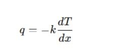
where:
- q is the heat flux,
- k is the thermal conductivity,
- dT/dx is the temperature gradient.
The heat transfer problem we consider here involves touching different materials at a given temperature. The perceived temperature at the skin surface differs based on the thermal conductivity (k) and thermal properties (ρcp) of the material.
Riemann-Temperature Expression
The Riemann-temperature expression estimates the temperature at the skin surface when a material is touched. It is given by:
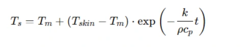
where:
This expression helps determine why some materials (like steel) feel colder than others (like concrete), even when both are at the same temperature.
2. Approach to Solving Similar Heat Transfer Assignments Using MATLAB
To solve similar assignments, follow these steps:
Understanding the Problem Statement
Before starting any MATLAB-based heat transfer assignment, the first step is to thoroughly understand the problem. This involves carefully analyzing the given data, identifying material properties, and understanding what is required. In most cases, assignments will provide the thermal conductivity (k) and volumetric heat capacity (ρcp) of the materials involved. Additionally, initial conditions such as the starting temperature of the materials and the skin must be noted. Another critical aspect is understanding the governing equation—such as the Riemann-temperature expression—which defines how heat transfer occurs when a material is touched. Clearly defining these elements ensures that the correct approach is followed in MATLAB.
Writing MATLAB Code for Computation
Once the problem statement is well understood, the next step is to translate the mathematical formulation into MATLAB code. This involves defining material properties using variables, setting up initial temperature values, and implementing the relevant heat transfer equations. MATLAB provides efficient tools for handling mathematical computations, making it easier to work with arrays and functions. Instead of manually computing values for different time steps, MATLAB allows automation through vectorized operations, loops, or built-in functions. The script should be structured to first define constants, then apply the formula to compute temperature changes over time, and finally, store or display the results for interpretation. Writing modular code—such as defining separate functions for calculations—makes it easier to reuse and adapt the script for different materials or scenarios.
Interpreting the Results
After executing the MATLAB script, analyzing the results is crucial. The computed skin surface temperatures for different materials over time reveal how quickly the perceived temperature stabilizes. In many cases, materials with higher thermal conductivity, such as metals, cause a more rapid drop in skin temperature, making them feel colder even at the same initial temperature. On the other hand, materials like concrete, which have lower thermal conductivity, do not conduct heat away from the skin as quickly, making them feel relatively warmer. Graphical visualization using MATLAB’s plotting functions enhances understanding by providing a clear comparison of how different materials affect temperature perception. By interpreting these results, students can draw meaningful conclusions about heat transfer properties and apply these concepts to various engineering applications.
3. MATLAB Implementation for Heat Transfer Assignments
Here’s how you can write a MATLAB script to solve this type of problem.
Step 1: Define Material Properties
Each material has a different thermal conductivity and heat capacity. Define these properties as variables:
% Define material properties
k_skin = 1;  % Thermal conductivity of skin (W/mK)
k_steel = 40; % Thermal conductivity of steel (W/mK)
k_concrete = 1; % Thermal conductivity of concrete (W/mK)

rho_cp_skin = 3.4e6; % Volumetric heat capacity of skin (J/m³K)
rho_cp_steel = 6e6; % Volumetric heat capacity of steel (J/m³K)
rho_cp_concrete = 2e6; % Volumetric heat capacity of concrete (J/m³K)
Step 2: Define Initial Conditions
Set the temperature of the materials and the skin before contact.
T_m = 0;  % Material temperature in °C
T_skin = 32;  % Skin temperature in °C
t = 0:0.1:5;  % Time in seconds (from 0 to 5 seconds)
Step 3: Compute the Perceived Temperature
Use the Riemann-temperature expression to compute the temperature at the skin surface.
% Function to calculate perceived temperature
T_s_steel = T_m + (T_skin - T_m) * exp(-k_steel ./ rho_cp_steel .* t);
T_s_concrete = T_m + (T_skin - T_m) * exp(-k_concrete ./ rho_cp_concrete .* t);
Step 4: Plot the Results
Visualizing the results helps in understanding how different materials affect the perceived temperature.
figure;
plot(t, T_s_steel, 'r', 'LineWidth', 2);
hold on;
plot(t, T_s_concrete, 'b', 'LineWidth', 2);
xlabel('Time (s)');
ylabel('Temperature at Skin Surface (°C)');
title('Perceived Temperature Over Time for Different Materials');
legend('Steel', 'Concrete');
grid on;
4. Generalizing for Similar Problems
The approach used in this guide is not limited to just steel and concrete; it can be easily adapted for different materials and conditions. In many assignments, students may be required to analyze heat transfer for materials such as wood, aluminum, glass, or polymers. The key to solving these problems is to first identify the given thermal properties and initial conditions, then apply the same Riemann-temperature expression. In MATLAB, modifying the script to accommodate new materials is straightforward—simply change the thermal conductivity (k) and volumetric heat capacity (ρcp ) values accordingly. Additionally, students may encounter scenarios where they need to factor in varying environmental conditions, such as the presence of external heat sources or varying contact durations. By adjusting the MATLAB script to include these parameters, they can develop a more accurate model of heat transfer behavior. Furthermore, assignments may require the comparison of multiple materials at once, in which case MATLAB’s ability to handle arrays and vectorized operations can be utilized to compute results efficiently. The flexibility of this approach makes it a valuable tool for tackling various engineering and physics assignments related to heat transfer.
5. Common Mistakes and How to Avoid Them
Students often make several mistakes when working on heat transfer assignments in MATLAB. One of the most common errors is using incorrect units, which can lead to misleading results. For instance, if thermal conductivity is given in watts per meter-Kelvin (W/mK) but heat capacity is in different units, conversions must be made to maintain consistency. Another frequent mistake is misinterpreting the Riemann-temperature equation, particularly the role of time and material properties in heat transfer. Some students also struggle with MATLAB syntax, especially when using element-wise operations with vectors. Using loops instead of vectorized calculations can also slow down computations unnecessarily. To avoid these mistakes, it is important to carefully check units, test code with known values, and utilize MATLAB’s debugging tools. Ensuring proper visualization of results through well-labeled plots can also help in verifying the accuracy of calculations.
6. Practical Applications of This Concept
Understanding how different materials conduct heat and affect perceived temperature has numerous real-world applications. In thermal engineering, this concept is used to design better insulation materials that minimize unwanted heat transfer. Engineers working in biomedical applications use similar principles to design medical devices and instruments that remain comfortable to the touch, reducing the risk of burns or discomfort. In the construction industry, knowledge of heat conduction helps in selecting flooring materials that do not feel excessively cold, improving indoor comfort. This is why materials like carpet or wood are often preferred over tile or metal surfaces in residential settings. The automotive industry also applies heat transfer principles to improve passenger comfort, ensuring that seats, dashboards, and steering wheels do not become too hot or cold under varying weather conditions. Additionally, in electronics and computing, heat transfer analysis is used to design cooling systems for processors and other components to prevent overheating. By understanding and applying heat transfer concepts, students can contribute to advancements in multiple fields, making this knowledge highly valuable beyond academic assignments.
Conclusion
Solving heat transfer assignments in MATLAB requires a structured approach that includes understanding the problem, writing efficient MATLAB code, interpreting results, and avoiding common mistakes. By carefully analyzing the material properties and implementing the Riemann-temperature expression, students can compute the perceived temperature for various materials and gain valuable insights into heat conduction. MATLAB’s powerful computational and visualization tools make it easier to solve and analyze such problems efficiently. By following these steps, students can confidently tackle similar assignments, modify their code for different materials, and strengthen their understanding of thermal physics and engineering applications.