Statistical Methods in Medical Research Assignment Help Using MATLAB

Making inferences about the variance of a sample based on the chi squared distribution assumes that the sample is normally distributed. When analyzing means, we were able to violate the assumption of normality because the central limit theorem states that the mean’s sampling distribution is normal. However, there is no central limit theorem for variance. In this question you will us the bootstrap method to make an inference about the variance of non-normally distributed data.

An Arteriosonde machine “prints” blood-pressure readings on a tape so that the measurement can be read rather than heard. A major argument for using such a machine is that the variability of measurements obtained by different observers on the same person will be lower than with a standard blood-pressure cuff. Extensive testing has shown that the traditional blood-pressure cuff has a variance of 3.7 mmHg2 between observers. You wish to show that the Arteriosonde machine has a lower variance between observers when compared to a traditional blood-pressure cuff.

Data for two observers making blood pressure readings on 50 individuals is presented in the file ‘BP_data.xlsx’

1. Provide evidence that you are not able to run a traditional chi-square distribution-based-test on the variance of the differences between the two observer’s blood pressure readings. Include a normal probability plot and a hypothesis test.

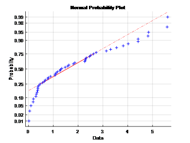
Ans: The normal probability plot does not follow a straight line which indicates the variance of the differencesbetween the two observer’s blood pressureis not a normal distribution. Furthermore, the application of t-test gives the h=1 which means it reject the null hypothesis that the variance of BP difference belongs to normal distribution.

2. Create 2,000 bootstrap samples by sampling with replacement from the differences between the two observer’s blood pressure readings. Do not include the bootstrap sample data here (there are too many values). Use your bootstrap samples to create a two-sided 95% bootstrap confidence interval on the variance of the differences between the two observer’s blood pressure readings. Include your CI here.

Ans: The CI interval is [1.4337, 2.2967].

3. Use this confidence interval to determine if the Arteriosonde machine produces a variance between the observer’s blood pressure readings that is below the 3.7 mmHg2 value for the traditional blood pressure cuff.

Ans: Both the upper and lower limits of CI is below 3.7 mmHg2 value.

4. Run a hypothesis test to determine if there are differences between the mean blood pressure measurements made by observer 1 and 2.

a. Include a p-value and 95% CI here:

Ans: The p-value= 0.0456and 95% CI =[0.1637, 3.5542].

b. Explain what your confidence interval means in the context of this problem.

Ans: The confidence interval means a significance level of 5%.

c. Explain why a parametric hypothesis test is appropriate even though the assumption of normality is violated.

Ans: The application of bootstrapping method to the BP data makes the use of parametric hypothesis testing appropriate.

Data and information for this problem sourced from:

Armitage P, Berry G. Statistical Methods in Medical Research. Blackwell: Oxford, 1987.

Data for birthweight (oz.) and weight at 70-100 days (oz.) of 14 babies are included in the file ‘birthweight.xlsx’.

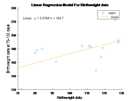
5. Create a simple linear regression model with birthweight as the regressor variable and weight at 70-100 days as the dependent variable. Plot this model and include your estimated value of β1.

6. It appears that there is a marginal relationship between birth weight and weight at 70-100 days. One way to confirm this relationship is to develop a confidence interval on β1. The data set is small, so we will use the bootstrap method to create at 95% CI on β1. Follow these steps to create your CI:

I. Randomly sample (with replacement) n=2000 cases.

II. Fit a linear regression model to the bootstrap samples to obtain the bootstrap slopesβ1*.

III. Use the empirical bootstrap method shown in class to create a 95% CI on bootstrap slopes.

a. Include the CI here:

Ans: The CI is [1.6651 1.6736]

b. Using your bootstrap CI as evidence, is there a statistically significant relationship between birthweight and weight at 70-100 days?

Ans: Due to excessive number of samples, the linear relationship between birthweight and weight at 70-100 days is destroyed so statistically significant relationship between them does not exist.

clc

clear all

close all

%%

%%%%%%%%% Task 1

data=readtable('BP_data.xlsx'); %%%% reading data from excelsheet

data=data{:,:}; %%%% converting table into matrix form

BP_obs1=data(:,2); %%%% BP data from observer 1

BP_obs2=data(:,3); %%%% BP data from observer 2

BP_diff=data(:,4); %%%% Difference BP data

normplot(BP_diff) %%%% Normal probability plot

[h,p]=ttest(BP_obs1,BP_obs2,'Alpha',0.01); %%%% application of paired t-test

%%

%%%%%% Task 2

n=2000; %%%% number of bootstrap samples

BP_diff_booted= bootstrp(2000,@mean,BP_diff);

CI = bootci(2000,@mean,BP_diff)

%%

%%%%%% Task 4

%%%%%%%%% Applying bootstrapping method to BP data

BP_obs1_booted= bootci(2000,@mean,BP_obs1);

BP_obs2_booted= bootci(2000,@mean,BP_obs2);

%%%% application of paired t-test with 5% significance level

[h,p,ci]=ttest(BP_obs1_booted,BP_obs2_booted,'Alpha',0.05)

Case 2 Code Solution

clc

clear all

close all

%%

%%%%%%%%% Task 1

data=readtable('birthweight.xlsx'); %%%% reading data from excelsheet

data=data{:,:}; %%%% converting table into matrix form

birthweight_pre=data(:,2); %%%% Birthweight data

birthweight_post=data(:,3); %%%% Birthweight data at 70-100 days

b=regress(birthweight_post,birthweight_pre) %%%% applying linear regression model to find coefficients

y_est= 0.6784.*birthweight_pre+104.7;

scatter(birthweight_pre,birthweight_post)

hold on

plot(birthweight_pre,y_est)

xlabel('Birthweight data')

ylabel('Birthweight data at 70-100 days')

title('Linear Regression Model For Birthweight data')

legend('data1','linear')

%%

%%%%%%% Task 2

n=2000; %%%% number of bootstrap samples

%%%%%% bootstrappinf data

birthweight_pre_booted= bootstrp(2000,@mean,birthweight_pre);

birthweight_post_booted= bootstrp(2000,@mean,birthweight_post);

[b, CI, ~, ~, stats]=regress(birthweight_post_booted,birthweight_pre_booted) %%%% applying linear regression model