Solving for f(omega) with pitzer’s acentric factor
The tables below highlights the Z factors for pressure from 50 to 6500 psia at temperature of 100 F.
| P (psia) | Z (100 F) | P (psia) | Z (100 F) |
| 50 | 0.97740 | 1500 | 0.48660 |
| 100 | 0.95450 | 1600 | 0.49510 |
| 200 | 0.90790 | 1700 | 0.50540 |
| 300 | 0.86000 | 1800 | 0.51690 |
| 400 | 0.81070 | 1900 | 0.52940 |
| 500 | 0.76010 | 2000 | 0.54240 |
| 600 | 0.70820 | 2500 | 0.61280 |
| 700 | 0.65580 | 3000 | 0.68660 |
| 800 | 0.60450 | 3500 | 0.76090 |
| 900 | 0.55770 | 4000 | 0.83510 |
| 1000 | 0.52020 | 4500 | 0.90860 |
| 1100 | 0.49540 | 5000 | 0.98160 |
| 1200 | 0.48260 | 5500 | 1.05390 |
| 1300 | 0.47860 | 6000 | 1.12560 |
| 1400 | 0.48060 | 6500 | 1.19670 |
| P (psia) | Z (200 F) | P (psia) | Z (200 F) |
| 50 | 0.98650 | 1500 | 0.70230 |
| 100 | 0.97300 | 1600 | 0.69730 |
| 200 | 0.94640 | 1700 | 0.69430 |
| 300 | 0.92020 | 1800 | 0.69330 |
| 400 | 0.89450 | 1900 | 0.69390 |
| 500 | 0.86950 | 2000 | 0.69610 |
| 600 | 0.84540 | 2500 | 0.72300 |
| 700 | 0.82240 | 3000 | 0.76610 |
| 800 | 0.80060 | 3500 | 0.81690 |
| 900 | 0.78030 | 4000 | 0.87150 |
| 1000 | 0.76190 | 4500 | 0.92810 |
| 1100 | 0.74540 | 5000 | 0.98570 |
| 1200 | 0.73110 | 5500 | 1.04380 |
| 1300 | 0.71920 | 6000 | 1.10210 |
| 1400 | 0.70960 | 6500 | 1.16050 |
MATLAB Script
% solving for f(omega) with the Pitzer’s acentric factor.
pitzer = [0.01330 0.11304 0.17244 0.23561 0.34585 0.55335 0.84182]
for i=1:7
if pitzer(i) <= 0.49
fomega(i)=0.374640+(1.54226*pitzer(i))-(0.26992*pitzer(i)^2)
else
fomega(i)=0.379642+(1.48503*pitzer(i))-(0.164423*pitzer(i)^2)+(0.016666*pitzer(i)^3)
end
end
% Attraction parameter constant,Co-volume parameter constant,binary interaction coefficients, mole fractions
omgai = [0.42312848 0.45192604 0.45984739 0.45811880 0.39778691 0.39778691 0.39778691]
omgbi = [0.08046461 0.07926051 0.07843675 0.07791799 0.07510754 0.07510754 0.07510754]
deltam=[0 0.000986 0.007843 0.023942 0.037841 0.047445 0.26562214;
0.000986 0 0.003695 0.010541 0.010541 0.010541 0.010541;
0.007843 0.003695 0 0.002281 0.002281 0.002281 0.002281;
0.023942 0.010541 0.002281 0 0.000 0.000 0.000;
0.037841 0.010541 0.002281 0.000 0 0.000 0.000;
0.047445 0.010541 0.002281 0.000 0.000 0 0.000;
0.26562214 0.010541 0.002281 0.000 0.000 0.000 0]
molef=[0.679300 0.099000 0.110800 0.045000 0.052966 0.011941 0.000993]
% getting critical temperature and solving for reduced temperature
TciF=[-120.01 89.83 245.87 410.94 600.51 823.88 1060.94]
TciR=TciF + 460
pci=[662.81 752.19 581.03 481.06 385.00 253.07 174.67]
% setting gas constant to units of psia and R
R = 10.7316
T1=100+460
T2=200+460
TrR=TciR.\T1
% dimensional attraction
for i=1:7
aalpha(i)= ((omgai(i)*(R^2)*(TciR(i)^2))/pci(i))*((1+((fomega(i)*(1-(TrR(i))^0.5))))^2);
end
% dimensional co-volume
for i=1:7
beta(i)= (omgbi(i)*R*TciR(i))/pci(i);
end
% enitre mixture parameters
aam = 0.0;
bm = 0.0;
for i=1:7
bm = bm + molef(i)*beta(i);
for j=1:7
aam=aam+molef(i)*molef(j)*sqrt( aalpha(i)*aalpha(j) )*(1.0-deltam(i,j));
end
end
% setting pressure
P=[50 100 200 300 400 500 600 700 800 900 1000 1100 1200 1300 1400 1500 1600 1700 1800 1900 2000 2500 3000 3500 4000 4500 5000 5500 6000 6500]
%solving for A, B, a1, b1, and c1 at temperature 560 R.
for i=1:30
A=(aam*P(i))/(R^2*T1^2);
B=(bm*P(i))/(R*T1);
a1=-(1-B);
b1=A-(3*B.^2)-(2*B);
c1=-((A.*B)-(B.^2)-(B.^3));
%solve for the roots
root1=roots([1 a1 b1 c1]);
RR(i) = root1(real(root1) >= 0 & imag(root1) == 0); %selecting positive real roots
end
%Repeat for temperature of 660 R.
TrR2=TciR.\T2
% dimensional attraction parameter
for i=1:7
aalpha2(i)= ((omgai(i)*(R^2)*(TciR(i)^2))/pci(i))*((1+((fomega(i)*(1-(TrR2(i))^0.5))))^2);
end
% dimensional co-volume parameters
for i=1:7
beta2(i)= (omgbi(i)*R*TciR(i))/pci(i);
end
% parameters for the entire mixture
aam2 = 0.0;
bm2 = 0.0;
for i=1:7
bm2 = bm2 + molef(i)*beta2(i);
for j=1:7
aam2=aam2+molef(i)*molef(j)*sqrt( aalpha2(i)*aalpha2(j) )*(1.0-deltam(i,j));
end
end
% setting pressure
P=[50 100 200 300 400 500 600 700 800 900 1000 1100 1200 1300 1400 1500 1600 1700 1800 1900 2000 2500 3000 3500 4000 4500 5000 5500 6000 6500]
%find A2, B2, a12, b12, and c12 at temperature of 660 R.
for i=1:30
A2=(aam2*P(i))/(R^2*T2^2);
B2=(bm2*P(i))/(R*T2);
a12=-(1-B2);
b12=A2-(3*B2.^2)-(2*B2);
c12=-((A2.*B2)-(B2.^2)-(B2.^3));
%solving for the roots
root2=roots([1 a12 b12 c12]);
RR2(i) = root2(real(root2) >= 0 & imag(root2) == 0); %select real positive values only
end
disp('Z factors for T=560 R ')
disp(RR)
disp('Z factors for T=660 R ')
disp(RR2)
%creating two plots
for i=1:30
x1(i)= P(i);
y1(i)= RR(i);
x2(i)= P(i);
y2(i)= RR2(i);
end
plot(x1, y1),xlabel('P(psia)'), ylabel('Z factor')
hold on
plot(x2, y2),xlabel('P(psia)'), ylabel('Z factor')
Graph
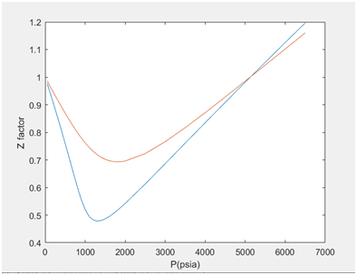
Figure 1: Z factor vs. P(psia) plot obtained from MATLAB for two temperatures plots, blue plot (100 F), orange (200 F).
MATLAB Script Output
>> zfactor_final
pitzer =
0.0133 0.1130 0.1724 0.2356 0.3458 0.5534 0.8418
fomega =
0.3951
fomega =
0.3951 0.5455
fomega =
0.3951 0.5455 0.6326
fomega =
0.3951 0.5455 0.6326 0.7230
fomega =
0.3951 0.5455 0.6326 0.7230 0.8757
fomega =
0.3951 0.5455 0.6326 0.7230 0.8757 1.1539
fomega =
0.3951 0.5455 0.6326 0.7230 0.8757 1.1539 1.5232
omgai =
0.4231 0.4519 0.4598 0.4581 0.3978 0.3978 0.3978
omgbi =
0.0805 0.0793 0.0784 0.0779 0.0751 0.0751 0.0751
deltam =
0 0.0010 0.0078 0.0239 0.0378 0.0474 0.2656
0.0010 0 0.0037 0.0105 0.0105 0.0105 0.0105
0.0078 0.0037 0 0.0023 0.0023 0.0023 0.0023
0.0239 0.0105 0.0023 0 0 0 0
0.0378 0.0105 0.0023 0 0 0 0
0.0474 0.0105 0.0023 0 0 0 0
0.2656 0.0105 0.0023 0 0 0 0
molef =
0.6793 0.0990 0.1108 0.0450 0.0530 0.0119 0.0010
TciF =
1.0e+03 *
-0.1200 0.0898 0.2459 0.4109 0.6005 0.8239 1.0609
TciR =
1.0e+03 *
0.3400 0.5498 0.7059 0.8709 1.0605 1.2839 1.5209
pci =
662.8100 752.1900 581.0300 481.0600 385.0000 253.0700 174.6700
R =
10.7316
T1 =
560
T2 =
660
TrR =
1.6471 1.0185 0.7933 0.6430 0.5280 0.4362 0.3682
P =
Columns 1 through 8
50 100 200 300 400 500 600 700
Columns 9 through 16
800 900 1000 1100 1200 1300 1400 1500
Columns 17 through 24
1600 1700 1800 1900 2000 2500 3000 3500
Columns 25 through 30
4000 4500 5000 5500 6000 6500
TrR2 =
1.9412 1.2004 0.9350 0.7578 0.6223 0.5141 0.4339
P =
Columns 1 through 8
50 100 200 300 400 500 600 700
Columns 9 through 16
800 900 1000 1100 1200 1300 1400 1500
Columns 17 through 24
1600 1700 1800 1900 2000 2500 3000 3500
Columns 25 through 30
4000 4500 5000 5500 6000 6500
Z factors for T=560 R
Columns 1 through 10
0.9774 0.9545 0.9079 0.8600 0.8107 0.7601 0.7082 0.6558 0.6045 0.5577
Columns 11 through 20
0.5202 0.4954 0.4826 0.4786 0.4806 0.4866 0.4951 0.5054 0.5169 0.5294
Columns 21 through 30
0.5424 0.6128 0.6866 0.7609 0.8351 0.9086 0.9816 1.0539 1.1256 1.1967
Z factors for T=660 R
Columns 1 through 10
0.9865 0.9730 0.9464 0.9202 0.8945 0.8695 0.8454 0.8224 0.8006 0.7803
Columns 11 through 20
0.7619 0.7454 0.7311 0.7192 0.7096 0.7023 0.6973 0.6943 0.6933 0.6939
Columns 21 through 30
0.6961 0.7230 0.7661 0.8169 0.8715 0.9281 0.9857 1.0438 1.1021 1.1605
>>