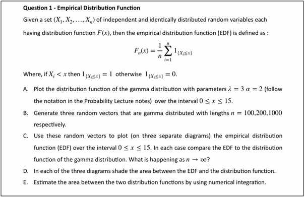
Empirical Distribution Function
MATLAB Script
clc, clear all, close all
%% Question 1
%% part A)
lambda = 3;
alpha = 2;
xspan = linspace(0, 15, 1000); % 1000 points between 0 and 15
n = length(xspan);
% Generate data X
X = rand(1,n)*15;
% Generate F_n (x)
F = zeros(n);
for xi = xspan
fori = 1:n
if X(i) <= xi
l = 1;
else
l = 0;
end
F(i) = F(i) + l;
end
end
F = 1/n *F;
% Calculate gamma distrbution
f = zeros(n,1);
fori = 1:n
xi = xspan(i);
if xi > 0
f(i) = (lambda^alpha)*xi^(alpha-1) *exp(-lambda*xi)/gamma(alpha);
else
f(i) = 0;
end
end
figure
plot(xspan, f), grid on
xlabel('X');
ylabel('Value');
title('Gamma Distribution');
%% part B)
x1 = rand(1,100);
x2 = rand(1,200);
x3 = rand(1,1000);
%% Part C)
% Empirical distributions
F = zeros(n);
fori = 1:n
Xi = X(i);
if Xi
F = F + 1;
end
end
% Generate F_n (x)
F1 = zeros(100,1);
xspan1 = linspace(0, 15, 100);
for xi = xspan1
fori = 1:100
if x1(i) <= xi
l = 1;
else
l = 0;
end
F1(i) = F1(i) + l;
end
end
F1 = 1/100 *F1;
% Calculate gamma distrbution
f1 = zeros(100,1);
fori = 1:100
xi = xspan1(i);
if xi > 0
f1(i) = (lambda^alpha)*xi^(alpha-1) *exp(-lambda*xi)/gamma(alpha);
else
f1(i) = 0;
end
end
F2 = zeros(200,1);
xspan2 = linspace(0, 15, 200);
for xi = xspan2
fori = 1:200
if x2(i) <= xi
l = 1;
else
l = 0;
end
F2(i) = F2(i) + l;
end
end
F2 = 1/200 *F2;
% Calculate gamma distrbution
f2 = zeros(200,1);
fori = 1:200
xi = xspan2(i);
if xi > 0
f2(i) = (lambda^alpha)*xi^(alpha-1) *exp(-lambda*xi)/gamma(alpha);
else
f2(i) = 0;
end
end
F3 = zeros(1000,1);
xspan3 = linspace(0, 15, 1000);
for xi = xspan3
fori = 1:1000
if x3(i) <= xi
l = 1;
else
l = 0;
end
F3(i) = F3(i) + l;
end
end
F3 = 1/1000 *F3;
% Calculate gamma distrbution
f3 = zeros(1000,1);
fori = 1:1000
xi = xspan3(i);
if xi > 0
f3(i) = (lambda^alpha)*xi^(alpha-1) *exp(-lambda*xi)/gamma(alpha);
else
f3(i) = 0;
end
end
% Plot
figure
subplot(3,1,1)
plot(xspan1, F1), grid on
hold on
plot(xspan1, f1)
title('n = 100')
subplot(3,1,2)
plot(xspan2, F2), grid on
hold on
plot(xspan2, f2)
title('n = 200')
subplot(3,1,3)
plot(xspan3, F3), grid on
hold on
plot(xspan3, f3)
title('n = 1000')
%%%%%%%%%%%%%%%%%%%%%%%%%%%%%%%%%%%%%%%%%
%% It can be seen that, as n increases, the "dispersion" between the points decreases, and the curve becomes a straight line with a negative slope
%%%%%%%%%%%%%%%%%%%%%%%%%%%%%%%%%%%%%%%%%
%% Part D)
shaded1 = [F1', fliplr(f1')];
xs1 = [xspan1, fliplr(xspan1)];
shaded2 = [F2', fliplr(f2')];
xs2 = [xspan2, fliplr(xspan2)];
shaded3 = [F3', fliplr(f3')];
xs3 = [xspan3, fliplr(xspan3)];
subplot(3,1,1)
fill(xs1, shaded1, 'y');
subplot(3,1,2)
fill(xs2, shaded2, 'y');
subplot(3,1,3)
fill(xs3, shaded3, 'y');
%% Part E)
fprintf("The area between the shaded region for n = 100 is: %.4f\n", trapz(xs1, shaded1));
fprintf("The area between the shaded region for n = 200 is: %.4f\n", trapz(xs2, shaded2));
fprintf("The area between the shaded region for n = 1000 is: %.4f\n", trapz(xs3, shaded3));
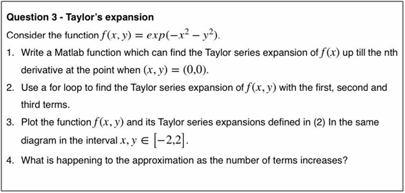
Taylor’s Expansion
Question 2 Solution
clc, clear all, close all
syms x y
f(x,y) = exp(-x^2 - y^2);
%% Part 1: Function in TaylorExpansion.m
T(x,y) = TaylorExpansion(f, 3);
%% part 2
for n = 0:3
fprintf("The Taylor Expansion for %d terms is:\n", n);
T(x,y) = TaylorExpansion(f, n)
end
%% Part 3
xspan = linspace(-2, 2, 50);
yspan = linspace(-2, 2, 50);
figure
hold on
legends = {};
for n = 0:6
T(x,y) = TaylorExpansion(f, n);
plot3(xspan, yspan, double(T(xspan, yspan)));
legends{n+1} = sprintf("%d terms\n", n);
end
legend(legends);
xlabel('X');
ylabel('Y');
zlabel('Z');
grid minor
view(3)
%% In the first terms, the function looks like a straight line on the X-Y plane. However, as n increases. the function
% becomes a polynomial that depends of both x and y. and it has the shape
% of a W. As n increases, the value of the curve decreases, but it
% maintains its shape.
Taylor’s SeriesExpansion Function
function T = TaylorExpansion(f, n)
syms x y
a = 0;
b = 0;
T(x,y) = sym(0);
forni = 0:n-1
fornj = 0:n-1
T(x,y) = T(x,y) + ((x-a)^ni)*((y-b)^(nj))/(factorial(ni)*factorial(nj)) *subs(diff(diff(f,y,nj),x,ni), [x,y], [0,0]);
end
end
end