Mass Conservation Equations
1. A stirred vessel is used to reduce the concentration of a contaminant in a liquid by adsorption onto particles of activated carbon. Its operation can be described by the following mass conservation equations
dC
dt = –K1(qeq – q)
dq
dt = K2(qeq – q)
Where C (in kg m–3) is the concentration of the contaminant in the liquid and q (in kg kg–1) is the quantity of contaminant adsorbed onto the activated carbon. qeq (in kg kg–1) is the equilibrium concentration adsorbed onto the activated carbon given by a piecewise-defined adsorption isotherm
8 qeq = 0.35C C 5 kg m–3
1 + 0.75C
< qeq = 0.246C0.25 C > 5 kg m–3
:
The model parameters are K1 = 5 10–2 kg m–3 s–1 and K2 = 5 10–4 s–1. At t = 0 s,
C = 50 kg m–3 and q = 0 kg kg–1.
Question 1 Solution
clc, clear all, close all
%% Question 1
K1 = 5e-2;
K2 = 5e-4;
C = 50;
q = 0;
% Define initial condition
C0 = 50;
q0 = 0;
% Define time of somulation and step
tf = 1*3600; % 3600 seconds or 1 hour
N = 10000; % Number of points to use for the time window
tspan = linspace(0, tf, N); % 10000 points between 0 and 3600
[t, x] = ode45(@(t,x)[-K1*(qeq(x(1))-x(2));K2*(qeq(x(1)) - x(2))], tspan, [C0, q0]);
C = x(:,1);
q = x(:,2);
% Plot solution
figure
subplot(1,2,1)
plot(tspan, C)
xlabel('Time (s)')
ylabel('{C(t)}')
grid on
title('{C(t) vs. time}')
subplot(1,2,2)
plot(tspan, q), grid on
xlabel('Time (s)')
ylabel('{q(t)}')
title('{q(t) vs. time}')
% Display the values at t = 1h in COmmand Window
fprintf("The value of C(t) at t = 1 h is: %.4f kg/m^3\n", C(end));
fprintf("The value of q(t) at t = 1 h is: %.4f kg/kg\n", q(end));
a. Develop a function in MATLAB that takes values of C as input argument and returns values of qeq as output according to the adsorption isotherm.
[5 marks]
1(a) Solution
function ret = Question1a_10601875(C)
% This function is for Question 1, Part a)
if C <= 5
ret = 0.35*C/(1+0.75*C);
else % C > 5
ret = 0.246*C^(0.25);
end
end
MATLAB Graph to Represent Evolution of the Concentration
b. Develop a program in MATLAB to represent graphically the evolution of the concentration of the contaminant in the liquid during the first hour of operation. The plot should have appropriate labels in both axes with SI units. The program should also write in the Command Window the value of the adsorbed concentration at t = 1 h, indicating as well the SI units.
[20 marks]
1(b) Solution
clc, clear all, close all
%% Question 1
K1 = 5e-2;
K2 = 5e-4;
% Define initial condition
C0 = 50;
q0 = 0;
% Define time of somulation and step
tf = 1*3600; % 3600 seconds or 1 hour
N = 10000; % Number of points to use for the time window
tspan = linspace(0, tf, N); % 10000 points between 0 and 3600
[t, x] = ode45(@(t,x)[-K1*(Question1a_10601875(x(1))-x(2));K2*(Question1a_10601875(x(1)) - x(2))], tspan, [C0, q0]);
C = x(:,1);
q = x(:,2);
% Plot solution
figure
subplot(1,2,1)
plot(tspan, C)
xlabel('Time (s)')
ylabel('{C(t)}')
grid on
title('{C(t) vs. time}')
subplot(1,2,2)
plot(tspan, q), grid on
xlabel('Time (s)')
ylabel('{q(t)}')
title('{q(t) vs. time}')
% Display the values at t = 1h in COmmand Window
fprintf("The value of C(t) at t = 1 h is: %.4f kg/m^3\n", C(end));
fprintf("The value of q(t) at t = 1 h is: %.4f kg/kg\n", q(end));
Van Der Waals Equation of State
2. The van der Waals equation of state is used by chemical engineers to predict properties of fluids. It is given by
p = RT – a
v – b v2
Where p is the pressure (in Pa), T the absolute temperature (in K) and v the molar volume of the fluid (in m3 mol–1). The parameter R = 8.314 J K–1 mol–1 is the ideal gas constant, and a = 3pcvc2 and b = vc/3 are model parameters, where vc and pc are the molar volume and pressure of the fluid at the critical point conditions, respectively.
The p – v curve for methane at T = 128 K is shown in Figure 2.1. For this compound, pc = 4.6 106 Pa and vc = 9.86 10–5 m3 mol–1. The vapour pressure, pvap, is defined as the pressure at which the areas A1 and A2 are equal (see Figure 2.1).
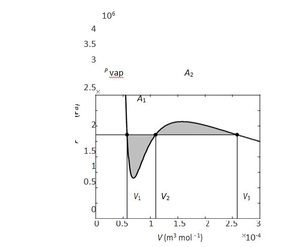
Figure 2.1: van der Waals isotherm for methane at T = 128 K.
a. The van der Waals equation can be expressed in polynomial form as
pv3 – (pb + RT )v2 + av = ab
Develop a MATLAB program to calculate the three possible solutions for the molar volume at a given value of pressure and T = 128 K. The program should return the three values in the Command Window with their SI units.
Hint: The three values can be calculated simultaneously using a particular built-in MATLAB function.
2(a) Solution [5 marks]
clc
clear all
%% Question 2, Part a)
R = 8.314; % ideal gas constant (J/k/mol)
pc = 4.6e6; % Pa
vc = 9.86e-5; % m^3 /mol
T = 128; % in Kelvin
% Calculate a and b
a = 3*pc*vc^2;
b = vc/3;
% Define the value of pressure (pavp)
p = 2.75e6;
% Calculate using roots function
% pv^3 - (pb+RT)v^2 + av - ab
v = roots([p, -(p*b + R*T), a, -a*b]);
fprintf("The three values of volume for T = %.0fK and p = %d Pa are:\n", T, p);
fprintf("v1 = %.6f m^3 /mol\nv2 = %.6f m^3 /mol\nv3 = %.6f m^3 /mol\n", v(1), v(2), v(3));
% Iterate v to get the graph of p vs. v
vspan = 0:1e-6:3e-4;
pspan = R*T./(vspan-b) - a./vspan.^2;
b. Develop a MATLAB function that takes as input argument a guess for the vapour pressure of methane at T = 128 K and returns the difference between the areas A1 and A2.
[10 mark]
Question 2(b) Solution
function ret = Question2b_10601875(p)
% Parameters
R = 8.314; % ideal gas constant (J/k/mol)
pc = 4.6e6; % Pa
vc = 9.86e-5; % m^3 /mol
T = 128; % in Kelvin
% Calculate a and b
a = 3*pc*vc^2;
b = vc/3;
% Calculate roots
v = roots([p, -(p*b + R*T), a, -a*b]);
% sort ascending
v = sort(v);
% Area A1 is between v(1) and v(2), area A2 is between v(2) and v(3)
N = 10000; % N equally-spaced points between intervals
h1 = (v(2)-v(1))/N;
h2 = (v(3)-v(2))/N;
vspan1 = v(1):h1:v(2);
vspan2 = v(2):h2:v(3);
p1 = R*T./(vspan1-b) - a./vspan1.^2;
p2 = R*T./(vspan2-b) - a./vspan2.^2;
% area under curve using trapz
A1 = trapz(vspan1, p1);
A2 = trapz(vspan2, p2);
% Difference in areas
ret = A2-A1;
end
c. Develop a program in MATLAB that uses the function developed in Question 2b to calculate the vapour pressure of methane at T = 128 K. The program should return the value of pvap in the Command Window with its SI units. Limit your search between the values of pressure 1.5 106 and 3 106 Pa.
Note: If you were not able to solve Question 2b, you can still solve Question 2c by assuming that you have a function named diffarea in the Current Folder that takes as input argument a guess for the vapour pressure of methane at T = 128 K and returns the difference between areas A1 and A2.
[10 marks]
2( C) Solution
clc
clear all
% Define limits of pressure
lb = 1.5e6;
ub = 3e6;
% Calculate difference in areas and select points for minimum difference
values = [];
pspan = lb:50:ub;
for p = pspan
Adiff = Question2b_10601875(p); % this is diffarea
values = [values, abs(Adiff)];
end
% Plot difference in areas
figure
plot(pspan, values)
grid on
xlabel('Pressure (Pa)');
ylabel('{|A_2-A_1|}')
title('Difference in areas');
[min_val, loc] = min(values);
fprintf("The pressure where the difference in areas is minimum is: %.0f Pa\n", pspan(loc))