How to Tackle and Solve Matlab Assignment on Double Pendulum

The study of dynamic systems is fundamental in physics and engineering, with the double pendulum being a well-known example of nonlinear motion and chaotic behavior. This system exhibits complex dynamics that make it an excellent subject for computational modeling. Many students face problem to complete their MATLAB assignment that require simulating and analyzing the motion of a double pendulum, which involves understanding its equations of motion and implementing numerical methods for solving them.
In this blog, we will break down the process into manageable steps. First, we will discuss the physical principles governing the double pendulum and derive the equations of motion. Next, we will explore how to transform these equations into a system of first-order differential equations suitable for numerical computation. We will then implement a fourth-order Runge-Kutta method in MATLAB to integrate the equations over time. Additionally, we will analyze the results by plotting key variables and observing how small changes in initial conditions can lead to vastly different outcomes due to the system's sensitivity.

By following this guide, you will develop a structured approach to solving similar MATLAB assignments, gaining confidence in handling numerical simulations, writing efficient code, and interpreting results in a meaningful way.
Step 1: Understanding the Double Pendulum System
A double pendulum consists of two rods connected end-to-end, each with a mass at its endpoint. The system exhibits complex motion and is sensitive to initial conditions, making it an interesting study in chaos theory. The motion of the system is governed by second-order differential equations, which we must solve numerically.
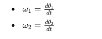
The two pendulums have angles θ1 and θ2, measured from the vertical. The corresponding angular velocities are ω1 = dθ1 / dt and ω2 = dθ2 / dt. The objective is to find θ1 (t) and θ2 (t) over time given initial conditions.
Derivation of Equations of Motion
The Lagrangian formulation provides a systematic way to derive the equations of motion for the double pendulum. The Lagrangian function is given by: L = T – V where T is the kinetic energy and V is the potential energy of the system.
For a double pendulum with masses m1 and m2, rod lengths L1 and L2, and gravitational acceleration g, the kinetic and potential energy expressions are:
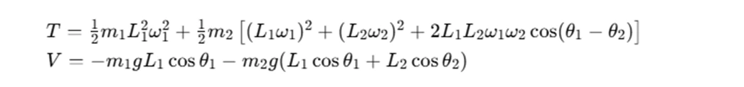
Applying the Euler-Lagrange equations, we obtain a system of second-order differential equations. To solve these equations numerically, we convert them into a system of first-order differential equations.
Step 2: Converting to First-Order System
Second-order differential equations can be rewritten as a system of first-order equations by defining angular velocities:
This allows us to express the system in the form y˙=f(y), where y=[θ1,θ2,ω1,ω2]. The function f(y) represents the system’s right-hand side, which we implement in MATLAB.
Implementing the Function in MATLAB
A MATLAB function to compute f(y) for the double pendulum can be written as follows:
function ydot = fpend(y)
    theta1 = y(1);
    theta2 = y(2);
    omega1 = y(3);
    omega2 = y(4);

    g = 1; L = 1; m = 1;

    delta = theta1 - theta2;
    den1 = (3 - cos(2*delta));
    den2 = den1;

    dOmega1 = (-3*sin(theta1) - sin(delta - 2*theta2) - 2*sin(delta) * (omega2^2 + omega1^2 * cos(delta))) / den1;
    dOmega2 = (2*sin(delta) * (2*omega1^2 + 2*cos(theta1) + omega2^2 * cos(delta))) / den2;

    ydot = [omega1; omega2; dOmega1; dOmega2];
end
This function takes a state vector y and returns its derivative.
Step 3: Implementing the Runge-Kutta Method
The fourth-order Runge-Kutta (RK4) method is commonly used for numerically integrating systems like this. The RK4 method provides better accuracy compared to Euler’s method.
MATLAB Implementation of RK4
function Y = runge_kutta(f, y0, t)
    h = t(2) - t(1);
    Y = zeros(length(t), length(y0));
    Y(1, :) = y0;

    for i = 1:length(t)-1
        k1 = f(Y(i, :))';
        k2 = f(Y(i, :) + 0.5 * h * k1)';
        k3 = f(Y(i, :) + 0.5 * h * k2)';
        k4 = f(Y(i, :) + h * k3)';
        Y(i+1, :) = Y(i, :) + (h/6) * (k1 + 2*k2 + 2*k3 + k4);
    end
end
This function numerically integrates a system using the RK4 method.
Step 4: Running Simulations with Different Initial Conditions
To observe different behaviors, we initialize the system with different values of θ1(0), θ2(0), ω1(0), and ω2(0).
t = 0:0.05:100;
y0 = [1, 1, 0, 0]; % Initial condition for Case 1
Y = runge_kutta(@fpend, y0, t);

theta2_vals = Y(:,2);
plot(t, theta2_vals);
xlabel('Time (s)');
ylabel('\theta_2 (t)');
title('Double Pendulum Motion');
grid on;
Step 5: Analyzing Step Size and Convergence
To analyze the accuracy of our method, we vary the step size h and compare results.
h_vals = [0.05, 0.025, 0.0125, 0.00625, 0.001];
errors = zeros(size(h_vals));

for i = 1:length(h_vals)
    t = 0:h_vals(i):100;
    Y = runge_kutta(@fpend, y0, t);
    errors(i) = abs(Y(end,2) - Y(end-1,2)); % Error in theta2 at t = 100
end

loglog(h_vals, errors, '-o');
xlabel('Step size (h)');
ylabel('Error');
title('Error vs Step Size');
grid on;
Conclusion
Solving a double pendulum assignment in MATLAB requires a structured approach, helping students develop practical skills in numerical integration, system modeling, and chaotic dynamics. The double pendulum is a classic example of nonlinear motion, making it an interesting yet challenging problem to solve. MATLAB offers robust tools for simulating and visualizing such complex systems, allowing students to explore the behavior of coupled differential equations.
To tackle this assignment effectively, students must first derive the system’s equations of motion and convert them into a first-order form. Implementing a numerical integration method, such as the fourth-order Runge-Kutta algorithm, enables accurate simulation of the pendulum’s movement over time. By experimenting with different initial conditions, students can observe the sensitivity of the system to small perturbations, a key characteristic of chaotic systems.
Additionally, refining the step size and analyzing the order of convergence help improve accuracy while reinforcing the importance of numerical stability. MATLAB’s visualization tools, such as animation functions, further enhance understanding by providing a dynamic representation of the pendulum’s motion. Through systematic experimentation and analysis, students gain valuable insights into differential equations, computational physics, and the power of MATLAB in solving real-world engineering problems.